Week 7 - Simulation of a 1D Super-sonic nozzle flow simulation using Macormack Method

WEEK 7 - SIMULATION OF A 1D SUPER-SONIC NOZZLE FLOW SIMULATION USING MAC CORMACK METHOD

AIM:

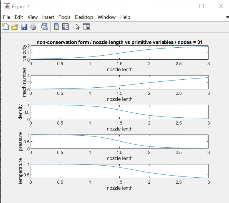
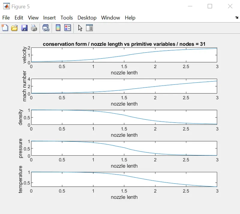
• Steady-state distribution of primitive variables inside the nozzle
• The code must be modular. You need to write separate functions to solve both forms.
• Discuss all the plots you are providing with observed inferences.
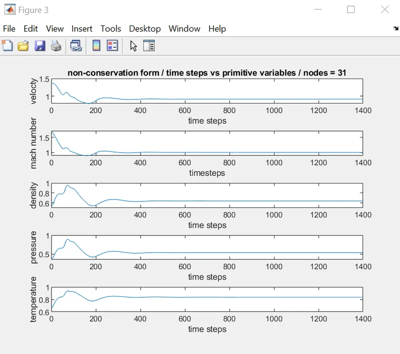
• Time-wise variation of the primitive variables.
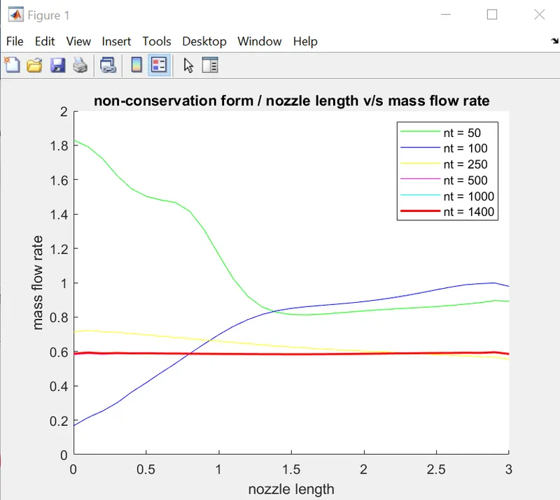
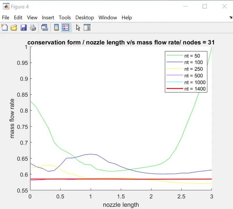
• Variation of Mass flow rate distribution inside the nozzle at different time steps during the time-marching process.
• Comparison of Normalized mass flow rate distributions of both forms.
  
  
  

THEORY:

Lagrangian approach:

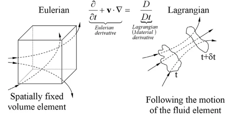
• Identify (or label) a material of the fluid; track (or follow) it as it moves, and monitor change in its properties. The properties may be velocity, temperature, density, mass, or concentration, etc in the flow field.
• Refer the above-figure. The ‘material’ or ‘particle’ of the fluid ‘A’ at time t has moved to some other location at time t’. Its property, say temperature, is recorded, as the material moves in the flow-field:

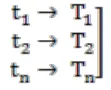
• Note that the recorded temperatures are associated with the same fluid particle, but at different locations and at different times.
• Think of a temperature sensor attached to a balloon, both having negligible mass and floating in the atmosphere and recording the atmosphere-temperature or the temperature of the flow-field. In such case, the following temperature-data are recorded by the sensor:

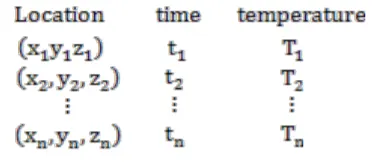
The time change of the temperature in such a measurement is denoted as DT/dt which is called material derivative or substantial derivative. It reflects time change in the temperature (or any other properties) of the labeled /marked/tagged fluid particles as observed by an observer moving with the fluid. Lagrangian approach is also called “particle based approach”.

Eulerian approach (a field approach):

• Identify (or label) a certain fixed location in the flow field and follow change in its property, as different materials pass through that location. In such case, the following property, say temperature is recorded by the sensor :

• Note that the recorded temperatures are associated with the fixed location in the flow-fluid, having
  different fluid elements at different times.
  
  
• The time- change of the temperature in such a measurement is denoted as which is
  called the partial derivativeof the temperature with respect to time. Note that the suffix (x,y,z) implies
  that the observer records the change in the property at the fixed location (x,y,z).

• is also called the local rate of change of that property (temperature in this case).

SUBSONIC - SUPERSONIC ISENTROPIC FLOW:

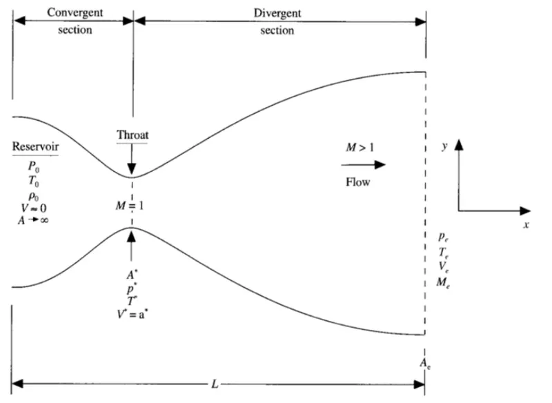
We consider the steady, isentropic flow through a convergent-divergent nozzle. The flow at the inlet to the nozzle comes from a reservoir where the pressure and temperature are denoted by p0 , and To, respectively. The cross-sectional area of the reservoir is large ( theoretically, A tends to infinity ), and hence the velocity is very small ( V tends to 0). Thus, Po and T0 are the stagnation values, or total pressure and total temperature respectively. The flow expands isentropically to supersonic speeds at the nozzle exit, where the exit pressure, temperature, velocity and Mach number are denoted by Pe, Te, Ve, and Me, respectlvely. The flow is locally subsonic in the convergent section of the nozzle, sonic at the throat (minimum area), and supersonic at the divergent sec1on. Te flow(M = 1) at the throat means that the local velocity at this location is equal to speed of sound.

DE-LAVAL NOZZLE:

GOVERNING EQUATIONS:

• we make the assumption that the flow properties-vary only with x; this is tantamount to assuming uniform flow properties across any given cross section. Such flow is defined as quasi-one-dimensional flow.
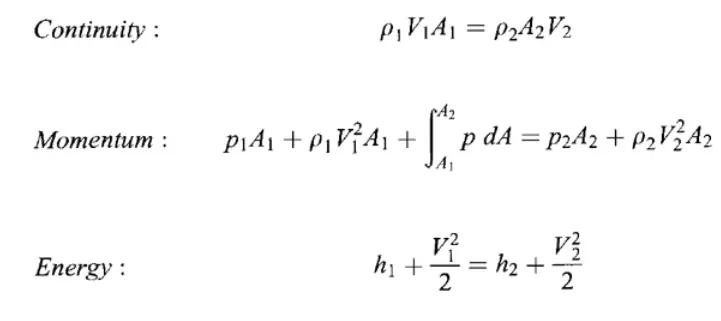
• The governing continuity, momentum, and energy equations for this quasi one-dimensional, steady, isentropic flow can be expressed, respectively, as

The Mach number variation through the nozzle is governed exclusively by the area ratio A/A* through the relation.

The pressure, density and temperature ratios are given by,

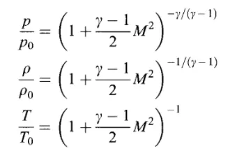
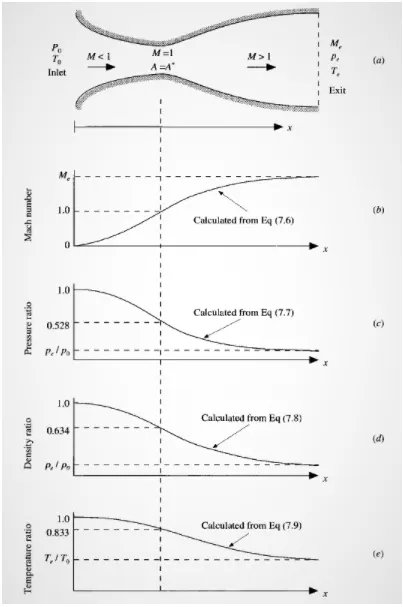
The variation of pressure, density, and temperature as a function of Mach number ( and hence as a function of Al A*, thus x) is given, respectively, by

MACCORMACK'S TECHNIQUE:

MacCormack's technique is a variant of the Lax-Wendroff approach but is much simpler in its application. Like the Lax-Wendroffmethod, the Maccormack method is also an explicit finite-difference technique which is second-order-accurate in both space and time. First introduced in 1969 (Ref. 43), it became the most popular explicit finite-difference method for solving fluid flows for the next 15 years. Today, the Maccormack method has been mostly supplanted by more sophisticated approaches. However, the Maccormack method is very "student friendly;" it is among the easiest to understand and program. Moreover, the results obtained by using MacCormack's method are perfectly satisfactory for many fluid flow applications.

CFD SETUP:

• The governing flow equations will be couched in terms of partial differentiatial equations suitable for the time marching solution of one-dimensional flow.
• The finite-difference expressions pertaining to Mac Cormack's technique as applied to this problem will be set-up.
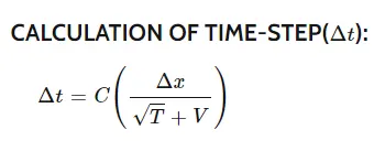
• Other details for numerical solution will be formulated such as calculation of time step and the treatment of boundary conditions.
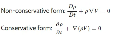
• Governing equations can be formulated in two forms.

1. conservative form

2. non-conservative form

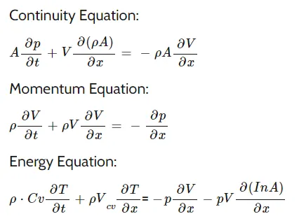
1. CONSERVATIVE FORM:

DISCRETISATION OF EQUATIONS:

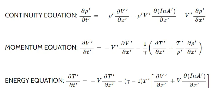
• The aabove mentioned equations set up the particular form of equations that will be most appropriate as well as convenient for time marching solution of quasi-one dimensional nozzle flow which consists of simplified form of solving PDE's.
• As second order degree equations are hard to solve, by the use of method, we get second order accurate time marching without much effort. So the, Mac Cormack's technique is an easy form of explicit finite-difference technique which is second order accurate in both space and time. It consists of

1. Predictor
2. Corrector

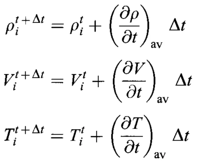
• We should start with predictor step, we should set the spatial derivatives up by the use of forward differencing scheme and the corrector step is done by the backward differencing scheme.
• Then we need to take the average of predictor and corrector method

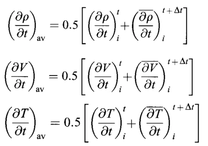
By using these below mentioned average values, we have to find the corrected values of the flow field variables at time t + dt. These steps should be repeated untill the steady state is reached.

NOZZLE SHAPE AND INITIAL CONDITIONS:

The nozzle shape, A = A(x) is specified and held fixed, independent of time, for the case illustrated in this section, we choose parabolic area distribution given by

Area variation along the nozzle

Hence, for our choice of initial conditions, they are chosen close to steady-state values so as to reduce the chances of the solution going unstable.

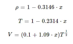
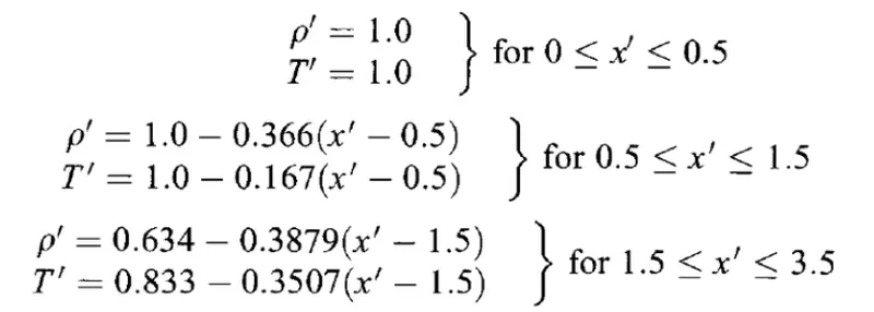
For simplicity, we are now assuming linear variations of the flow field variables, as a function of x. For the present case, we assume the followingvalues at t = 0

Density, temperature and velocity variation along the nozzle

BOUNDARY CONDITIONS:

Boundary conditions are important because the applicablity of numerical methods and the resultant quality of computations can critically be decided on how those are numerically treated and without proper implementation of boundary conditions and their numerically proper representation, we have no hope whatsover of obtainin a proper numerical solution to our flow problem.

SUBSONIC INFLOW BOUNDARY AT POINT 1:

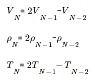
Here we are allowing one variable to float and we are choosing the velocity v1 because on a physical basis we know that mass flow rate flow through the nozzle must be allowed to adjust to the proper steady state and hence allowing variable velocity v1 to float makes the most sense as part of the adjustment. The value of v1 changes with respect to time and the information is obtained from flow field solution over the internal points. we are using linear extrapolation from point 2 and 3 to calculate v1 and take rho(1) = 1 and t(1) = 1 as fixed values.

SUPERSONIC INFLOW BOUNDARY AT POINT 1:

For this, we must allow all flow field variables to float. We are choosing to use linear extrapolation based on the flow field values at the internal point. Specially, we have the values for the non-dimensional variables.

CONSERVATIVE FORM:

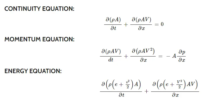
We need to convert these equations into non-dimensional form, so the converted equations are

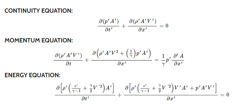
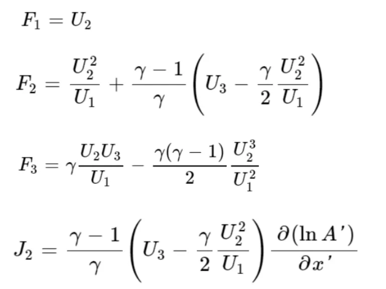
Lets express the equations for the quasi-one dimensional flow in generic form. we are going to define the solution vector U, the flux vector F, and the source term J as

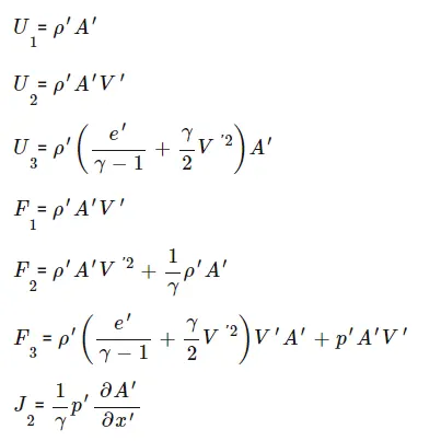
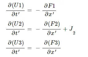
Now we need to substitute the below terms into the above equations

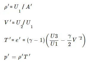
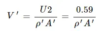
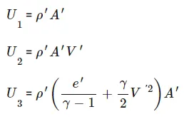
Now we need to obtain the primitive variables inorder to do that we must decode the elements U1, U2 and U3

Now we need to write the governing equations purely in terms of solution vectors.

PREDICTOR STEP:

To start the calculation, we are using the initial conditions for U1, U2 and U3 to calculate the initial values of F1, F2 and F3 and we use these values to calculate the values of U1, U2 and U3.

CORRECTOR STEP:

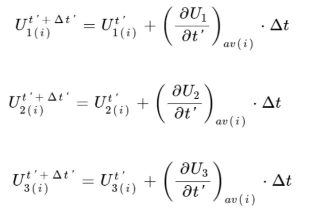
Now using the predicted values, we can calculate the new flux term and source terms. we are then calculating the time derivative terms by using backward difference and then we are calculating the average values of time derivatives of predictor and corrctor steps.

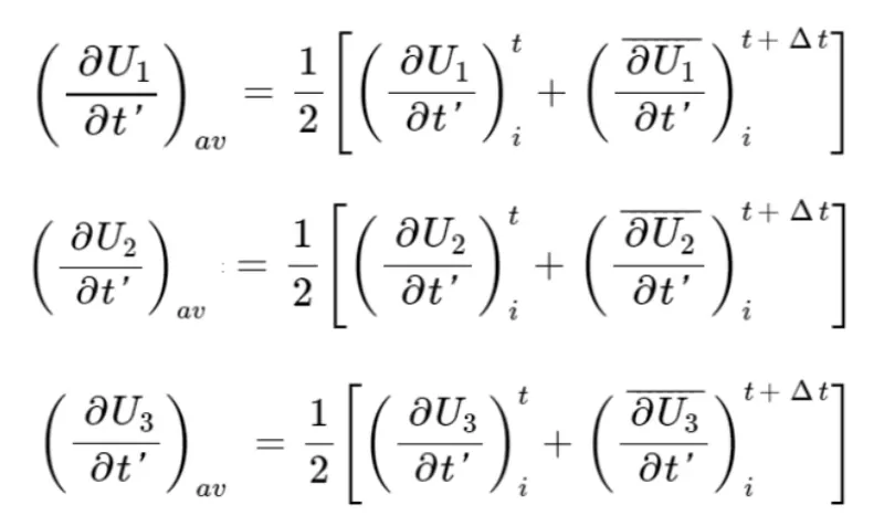
These steps are repeated untill the steady state is acieved.

INITIAL CONDITIONS:

BOUNDARY CONDITIONS:

SUBSONIC INFLOW BOUNDARY CONDITIONS AT POINT 1:

At the subsonic flow boundary, two properties are held fixed and one is allowed to float and at the supersonic flow boundary all properties are allowed to float.

SUBSONIC INFLOW BOUNDARY CONDITIONS AT POINT N:

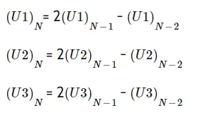
In the case of the supersonic outflow boundary, all properties are allowed to float. The flow properties at the downstream supersonic outflow boundary are obtained by linear extrapolation from the two adjacent internal points. If N denotes the grid point at the outflow boundary, then

PROGRAM CODE FOR NON-CONSERVATION FORM BY USING FUNCTION:

% function code for non- conservation form
function [rho,v,t,p,m,M_th,p_th,rho_th,t_th,x] = non_conservation(nt)

% inputs
n_NC = 31;
x = linspace(0, 3, n_NC);
dx = x(2) - x(1);


% calculate initial profiles
rho = 1 - (0.3146 * x);
t   = 1 - (0.2314 * x);
v   = (0.1 + 1.09 * x).* t.^0.5;

% area
a = 1 + ((2.2) * ((x - 1.5).^2));

% time steps
%  dt = 0.01;
gamma = 1.4;

% cfl_NC = max((v + sqrt(t)) * dt/dx)
cfl = 0.5

% time step
for s = 1:n_NC
    dt_NC_calc(s) = (cfl*dx)/(((t(s)).^0.5) + v(s));
end
dt = min(dt_NC_calc);

%outer time loop
for i = 1:nt

    rho_old = rho;
    v_old   = v;
    t_old   = t;

    % predictor method
    for j  = 2: n_NC-1
        % making the continuity into four parts to avoid complexity
        dv_dx      = (v(j+1)-v(j))/dx;
        d_rho_dx   = (rho(j+1)-rho(j))/dx;
        dt_dx      = (t(j+1)-t(j))/dx;
        d_log_a_dx = (log(a(j+1))-log(a(j)))/dx;

        % continuity equation
        d_rho_dt_p(j) = -rho(j) * dv_dx - rho(j) * v(j) * d_log_a_dx - v(j) * d_rho_dx;

        % momentum equation
        dv_dt_p(j) = -v(j) * dv_dx - (1/gamma) * (dt_dx + (t(j)/rho(j))*d_rho_dx);

        % energy equation
        dt_dt_p(j) = -v(j) * dt_dx - (gamma - 1) * t(j) * (dv_dx + v(j) * v(j) * d_log_a_dx);

        % solution update
        rho(j) = rho(j) + d_rho_dt_p(j) * dt;
        t(j)   = t(j) + dv_dt_p(j) * dt;
        v(j)   = v(j) + dv_dt_p(j) * dt;
    end

    % corrector method
    for j  = 2: n_NC-1
        % making the continuity into four parts to avoid complexity
        dv_dx      = (v(j)-v(j-1))/dx;
        d_rho_dx   = (rho(j)-rho(j-1))/dx;
        dt_dx      = (t(j)-t(j-1))/dx;
        d_log_a_dx = (log(a(j))-log(a(j-1)))/dx;

        % continuity equation
        d_rho_dt_c(j) = -rho(j) * dv_dx - rho(j) * v(j) * d_log_a_dx - v(j) * d_rho_dx;

        % momentum equation
        dv_dt_c(j) = -v(j) * dv_dx - (1/gamma) * (dt_dx + (t(j)/rho(j))*d_rho_dx);

        % energy equation
        dt_dt_c(j) = -v(j) * dt_dx - (gamma - 1) * t(j) * (dv_dx + v(j) * v(j) * d_log_a_dx);

    end
    % average derivative
    d_rho_dt = 0.5 * (d_rho_dt_p + d_rho_dt_c);
    dv_dt    = 0.5 * (dv_dt_p + dv_dt_c);
    dt_dt    = 0.5 * (dt_dt_p + dt_dt_c);

    % final solution update
    for k = 2:n_NC-1
        rho(k) = rho_old(k) + d_rho_dt(k) * dt;
        v(k)   = v_old(k) + dv_dt(k) * dt;
        t(k)   = t_old(k) + dt_dt(k) * dt;
    end

    % boundary conditions
    % inlet
    v(1) = 2 * v(2) - v(3);

    % outlet
    v(n_NC)   = 2 * v(n_NC-1) - v(n_NC-2);
    rho(n_NC) = 2 * rho(n_NC-1) - rho(n_NC-2);
    t(n_NC)   = 2 * t(n_NC-1) - t(n_NC-2);

    p = rho.*t;
    M = v./sqrt(t);
    m = rho.*a.*v;

    rho_th(i) = rho(16);
    v_th(i)   = v(16);
    t_th(i)   = t(16);
    p_th(i)   = p(16);
    M_th(i)   = M(16);

    figure(1)
    hold on

    if i == 50
        plot(x,m,'DisplayName','nt = 50','color','g')
    end

    if i == 100
        plot(x,m,'DisplayName','nt = 100','color','b')
    end

    if i == 250
        plot(x,m,'DisplayName','nt = 250','color','y')
    end

    if i == 500
        plot(x,m,'DisplayName','nt = 500','color','m')
    end

    if i == 1000
        plot(x,m,'DisplayName','nt = 1000','color','c')
    end

    if i == 2000
        plot(x,m,'DisplayName','nt = 2000','color','r','linewidth',1.5)
    end

end
title('non-conservation form / nozzle length v/s mass flow rate')
xlabel('nozzle length')
ylabel('mass flow rate')
legend

figure(2)
subplot(5,1,1)
plot(x,v)
xlabel('nozzle lenth')
ylabel('velocity')
title('non-conservation form / nozzle length vs primitive variables / nodes = 31')


subplot(5,1,2)
plot(x,M)
xlabel('nozzle lenth')
ylabel('mach number')

subplot(5,1,3)
plot(x,rho)
xlabel('nozzle lenth')
ylabel('density')

subplot(5,1,4)
plot(x,p)
xlabel('nozzle lenth')
ylabel('pressure')


subplot(5,1,5)
plot(x,t)
xlabel('nozzle lenth')
ylabel('temperature')

figure(3)
hold on
subplot(5,1,1)
plot(v_th)
xlabel('time steps')
ylabel('velocty')
title('non-conservation form / time steps vs primitive variables / nodes = 31')

subplot(5,1,2)
plot(M_th)
xlabel('timesteps')
ylabel('mach number')

subplot(5,1,3)
plot(rho_th)
xlabel('time steps')
ylabel('density')

subplot(5,1,4)
plot(p_th)
xlabel('time steps')
ylabel('pressure')

subplot(5,1,5)
plot(t_th)
xlabel('time steps')
ylabel('temperature')

end

STEP-WISE CODE EXPLANATION:

step-1:

Introduce the function format and include the variables which are used in the plots as outputs in left side of the format and mention the inputs in the right side of the format

step-2:

Mention the inputs suc as time steps, interval and nuber of nodes, were the nozzle length 3 metres is divided into 31 nodes equally

step-3:

We need to calculate the initial profiles of density, temperature, pressure, velocity and area of nozzle by using the equations given in J.D.Anderson book.

step-4:

Here we need to mention the cfl number and calculate the time step by using cfl number, temperature and velocity taking the minimum value of all te iterations by creating a loop.

step-5:

We need to create the time loop, inside this loop we need to mention the following from step six,

step-6:

We need to update the values of primitive variables as old.

step-7:

We need to use the predictor method and we need to divide governing equations such as continuity, momentum and energy into parts to avoid the complexity such as dv_dx, d_rho_dx, d_log_a_dx and dt_dx and next we need to update density, temperature and velocity by using the loop.

step-8:

Similarly we also need to do this for corrector method by using the loop.

step-9:

We need to take the average of both predictor and corrector method outside corrector loop and inside time loop.

step-10:

We need to create loop to calculate the final solution of primitive variables.

step-11:

We need to use the inlet and outlet boundary conditions for the problem which very important to get the good approximate solution

step-12:

Now we need to calculate the pressure and mach number using other primitive variables.

step-13:

Now we need to make the values of primitive variables at the throat point for all iterations which is alraedy calculated and it has to be used to plot the results.

step-14:

Now we need to plot the 3 graphs,

step-15:

plot-1:using the "if loop" we need to plot te nozzle length vs mass flow rate at different number of iterations.

step-16:

plot-2: using the plot and subplot command, we need to plot 5 graphs which are nozzle length vs 5 primitive variables

step-17:

plot-3: using the plot and subplot command, we need to plot 5 graphs which are time steps vs 5 primitive variables of throat.

PRORAM CODE FOR CONSERVATION FORM BY USING FUNCTION:

% function code for conservation form
function [rho,v,t,p,m,M_th,p_th,rho_th,t_th,x] = conservation(nt)

% inputs
n_C = 31
x = linspace(0, 3, n_C);
dx = x(2) - x(1);

% calculate initial profiles
rho = 1 - (0.3146 * x);
t   = 1 - (0.2314 * x);
v   = (0.1 + 1.09 * x).* t.^0.5;

% if iterative_solver == 2

% initial conditions
for z = 1:n_C

    if x(z)>=0 && x(z)<= 0.5
        rho(z) = 1;
        t(z)   = 1;
    end

    if x(z)>= 0.5 && x(z)<= 1.5
        rho(z) = 1 - 0.366 * (x(z) - 0.5);
        t(z)   = 1 - 0.167 * (x(z) - 0.5);
    end

    if x(z)>= 1.5 && x(z)<=3.5
        rho(z) = 0.634 - 0.3879 * (x(z) - 1.5);
        t(z)   = 0.833 - 0.3507 * (x(z) - 1.5);
    end
end

% area
a = 1 + ((2.2) * ((x - 1.5).^2));
v = 0.59./(rho.* a);
p = rho.* t;


% cfl_NC = max((v + sqrt(t)) * dt/dx)
cfl = 0.49

% time steps
for s = 1:n_C
    dt_C_calc(s) = (cfl*dx)/(((t(s)).^0.5) + v(s));
end

dt = min(dt_C_calc);
gamma = 1.4;


U1 = rho.* a;
U2 = rho.* a.* v;
U3 = U1.* ((t./(gamma - 1)) + ((gamma/2) * (v.^2)));



%outer time loop
for i = 1:nt

    %     rho_old = rho;
    %     v_old   = v;
    %     t_old   = t;

    U1_OLD = U1;
    U2_OLD = U2;
    U3_OLD = U3;

    F1 = U2;
    F2 = ((U2.^2)./U1) + (((gamma - 1)/gamma) * (U3 - ((gamma/2) * ((U2.^2)./U1))));
    F3 = ((gamma * U2.* U3)./U1) - ((0.5 * gamma * ((gamma - 1)) * U2.^3)./U1.^2);

    % predictor method
    for j = 2:n_C-1
        J2 = (1/gamma) * rho(j) * t(j) * ((a(j+1) - a(j))/dx);
        % continuity equation
        d_U1_dt_p(j) = -(F1(j+1) - F1(j))/dx;

        % momentum equation
        d_U2_dt_p(j) = -((F2(j+1) - F2(j))/dx) + J2;

        % energy equation
        d_U3_dt_p(j) = -(F3(j+1) - F3(j))/dx;

        % solution update of predictor method
        U1(j) = U1(j) +  (d_U1_dt_p(j) * dt);
        U2(j) = U2(j) +  (d_U2_dt_p(j) * dt);
        U3(j) = U3(j) +  (d_U3_dt_p(j) * dt);
    end

    % variables update
    rho = U1./a;
    v   = U2./U1;
    t   = (gamma - 1) * ((U3./U1) - ((gamma/2) * (v.^2)));
    p   = rho.* t;

    F1 = U2;
    F2 = ((U2.^2)./U1) + (((gamma - 1)/gamma) * (U3 - ((gamma/2) * ((U2.^2)./U1))));
    F3 = ((gamma * U2.* U3)./U1) - ((0.5 * gamma * ((gamma - 1)) * U2.^3)./U1.^2);


    % corrector method
    for j = 2:n_C-1
        J2 = (1/gamma) * rho(j) * t(j) * ((a(j) - a(j-1))/dx);
        % continuity equation
        d_U1_dt_c(j) = -(F1(j) - F1(j-1))/dx;

        % momentum equation
        d_U2_dt_c(j) = -((F2(j) - F2(j-1))/dx) + J2;

        % energy equation
        d_U3_dt_c(j) = -(F3(j) - F3(j-1))/dx;
    end

    % average of time derivative
    d_U1_dt = 0.5 * (d_U1_dt_c + d_U1_dt_p);
    d_U2_dt = 0.5 * (d_U2_dt_c + d_U2_dt_p);
    d_U3_dt = 0.5 * (d_U3_dt_c + d_U3_dt_p);

    % final solution update
    for k = 2:n_C-1
        U1(k) = U1_OLD(k) + (d_U1_dt(k) * dt);
        U2(k) = U2_OLD(k) + (d_U2_dt(k) * dt);
        U3(k) = U3_OLD(k) + (d_U3_dt(k) * dt);
    end

    % variables final update
    rho = U1./a;
    v   = U2./U1;
    t   = (gamma - 1) * ((U3./U1) - ((gamma/2) * (v.^2)));


    % inlet boundary conditions
    U1(1) = a(1);
    U2(1) = (2 * U2(2)) - U2(3);
    U3(1) = U1(1) * (t(1)/(gamma - 1) + (gamma/2) * v(1)^2);

    % outlet boundary conditions
    U1(n_C) = (2 * U1(n_C-1)) - U1(n_C-2);
    U2(n_C) = (2 * U2(n_C-1)) - U2(n_C-2);
    U3(n_C) = (2 * U3(n_C-1)) - U3(n_C-2);

    p = rho.*t;
    M = v./sqrt(t);
    m = rho.*a.*v;

    %     % at throat
    %     rho_th(i) = rho(16);
    %     v_th(i)   = v(16);
    %     t_th(i)   = t(16);
    %     p_th(i)   = p(16);
    %     M_th(i)   = M(16);

    % at throat
    rho_th(i) = rho(16);
    v_th(i)   = v(16);
    t_th(i)   = t(16);
    p_th(i)   = p(16);
    M_th(i)   = M(16);

    figure(4)
    hold on

    if i == 50
        plot(x,m,'DisplayName','nt = 50','color','g')
    end

    if i == 100
        plot(x,m,'DisplayName','nt = 100','color','b')
    end

    if i == 250
        plot(x,m,'DisplayName','nt = 250','color','y')
    end

    if i == 500
        plot(x,m,'DisplayName','nt = 500','color','m')
    end

    if i == 1000
        plot(x,m,'DisplayName','nt = 1000','color','c')
    end

    if i == 2000
        plot(x,m,'DisplayName','nt = 2000','color','r','linewidth',1.5)
    end

end

title('conservation form / nozzle length v/s mass flow rate/ nodes = 62')
xlabel('nozzle length')
ylabel('mass flow rate')
legend

% plots
figure(5)
subplot(5,1,1)
plot(x,v)
xlabel('nozzle lenth')
ylabel('velocity')
title('conservation form / nozzle length vs primitive variables / nodes = 62')

subplot(5,1,2)
plot(x,M)
xlabel('nozzle lenth')
ylabel('mach number')

subplot(5,1,3)
plot(x,rho)
xlabel('nozzle lenth')
ylabel('density')

subplot(5,1,4)
plot(x,p)
xlabel('nozzle lenth')
ylabel('pressure')


subplot(5,1,5)
plot(x,t)
xlabel('nozzle lenth')
ylabel('temperature')

figure(6)
hold on
subplot(5,1,1)
plot(v_th)
xlabel('time steps')
ylabel('velocty')
title('conservation form / time steps vs primitive variables / nodes = 62')

subplot(5,1,2)
plot(M_th)
xlabel('timesteps')
ylabel('mach number')

subplot(5,1,3)
plot(rho_th)
xlabel('time steps')
ylabel('density')

subplot(5,1,4)
plot(p_th)
xlabel('time steps')
ylabel('pressure')

subplot(5,1,5)
plot(t_th)
xlabel('time steps')
ylabel('temperature')
end

STEP-WISE CODE EXPLANATION:

step-1:

Introduce the function format and include the variables which are used in the plots as outputs in left side of the format and mention the inputs in the right side of the format

step-2:

Mention the inputs such as time steps, interval and nuber of nodes, were the nozzle length 3 metres is divided into 31 nodes equally.

step-3:

We need to calculate the initial profiles of density, temperature, pressure, velocity and area of nozzle and also some initial conditions, we need to assingn the 3 types of values at nozzle lengths of 0 - 0.5, 0.6 - 1.5, 1.6 - 3.5 with help of equations given in J.D.Anderson book.

step-4:

Here we need to mention the cfl number and calculate the time step by using cfl number, temperature and velocity taking the minimum value of all te iterations by creating a loop by using the equations given in J.D.Anderson book.

step-5:

We need to assign the terms called U1, U2, U3, F1, F2, F3 and J2.

step-6:

We need to create the outer time loop, inside this loop we need to mention the following from step seven,

step-7:

Again we need to add the above mentioned terms inside the outer time loop.

step-8:

We need to use the predictor method and we need to divide governing equations such as continuity, momentum and energy into parts to avoid the complexity such as dv_dx, d_rho_dx, d_log_a_dx and dt_dx and next we need to update density, temperature and velocity by using the loop.

step-9:

Now we need to update the primitive variables and F1, F2 and F3 outside the predictor method.

step-10:

Similarly we also need to do this for corrector method by using the loop.

step-11:

We need to take the average of both predictor and corrector method outside corrector loop and inside time loop.

step-12:

We need to create loop to calculate the final solution of primitive variables.

step-13:

We need to use the inlet and outlet boundary conditions for the problem which very important to get the good approximate solution

step-14:

Now we need to calculate the pressure and mach number using other primitive variables.

step-15:

Now we need to make the values of primitive variables at the throat point for all iterations which is alraedy calculated and it has to be used to plot the results.

step-16:

Now we need to plot the 3 graphs,

step-17:

plot-1:using the "if loop" we need to plot te nozzle length vs mass flow rate at different number of iterations.

step-18:

plot-2: using the plot and subplot command, we need to plot 5 graphs which are nozzle length vs 5 primitive variables

step-19:

plot-3: using the plot and subplot command, we need to plot 5 graphs which are time steps vs 5 primitive variables of throat.

MAIN PROGRAM CODE:

% main code for mac-cormack's method
close all
clear clc
clc

nt = 2000;

% non- conservation function
[rho_NC,v_NC,t_NC,p_NC,m_NC,M_th_NC,p_th_NC,rho_th_NC,t_th_NC,x_NC] = non_conservation(nt);

% conservation function
[rho_C,v_C,t_C,p_C,m_C,M_th_C,p_th_C,rho_th_C,t_th_C,x_C] = conservation(nt);

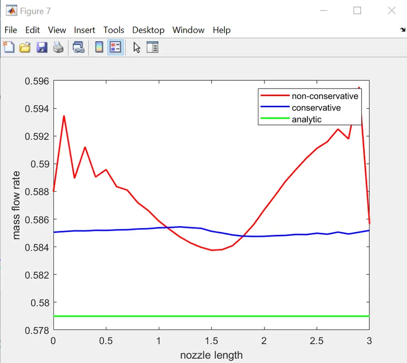
% mass flow rate comparision between conservative, non- conservative and analytic form
figure(7)

% non conservative plot
plot(x_NC,m_NC,"Color",'r',"LineWidth",1.5)
hold on

% conservative plot
plot(x_C,m_C,"Color",'b',"LineWidth",1.5)
hold on

% analytic plot
line([0,3],[0.579 0.579],"color",'g',"linewidth",1.5)
hold on
xlabel('nozzle length')
ylabel('mass flow rate')
legend('non-conservative','conservative','analytic')

STEP-WISE CODE EXPLANATION:

step-1:

We need to mention the number of iterations.

step-2:

we need to mention the function terms of conservative and non-conservative forms.

step-3:

we need to plot the figure of conservative, non-conservative and analytic for nozzle length vs mass flow rate.

RESULTS AND OUTPUT:

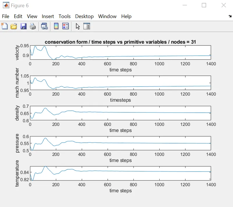
EXPLANATION OF RESULTS:

• From the comparision of mass flow rate for all the two forms of solutions with analytical solution, we can say that conservative form as a very good approximation of mass flow rate distribution compared to non-conservative form.
• The conservative form result is very much close to the analytic result, so we can say it is better than non-conservative form in tis pointof view.
• The only dis-advantae of this metohd is to write the code it takes so much time.
• From the graphs of primitive variables vs nozzle length, we can say that conservative form graphs are pretty much exact to analytic solution.
• Mac Cormack's method is best suitable for the nozzle problem compared to previous method which is Lax-Wendroff's method.
• If we increase the number of nodes, the solution will be further exact to analytic solution.