Week 3.5 - Deriving 4th order approximation of a 2nd order derivative using Taylor Table method
WEEK 3.5 - DERIVING 4TH ORDER APPROXIMATION OF A 2ND ORDER DERIVATIVE USING TAYLOR TABLE METHOD
Aim:
- To compute the given function.
- To compute the given second derivative.
- To compute the derivative both numerically and analytically of fourth order approximations.
- To derive and calculate all the three skewed right sided difference, left sided difference and centered difference approximations and by using absolute command.
- To calculate the errors of all the three approximations.
- To plot a bar graph with labels , legends and headings.
- To upload the file.
Theory:
1. skewed right - sided difference:
The number of nodes required for the 4th order aproximation of a second order derivative can be given by the equation N = P + Q = 2 + 4 + 6
where,
N - number of nodes
O - order of derivative
P - order of derivative
Hypothesis equation:
`(del^2f)/(delx)^2 = afi + bf(i+1) + cf(i+2) + df(i+3) + ef(i+4) + gf(i+5)`
from here we can say that totally 6 nodes are required to compute 4th order approximation of a second order derivative.
2. Skewed left sided difference:
N = P + Q = 2 + 4 = 6,
from here we can say that totally 6 nodes are required to compute 4th order approximation of a second order derivative.
`(del^2f)/(delx)^2 = afi + bf(i-1) + cf(i-2) + df(i-3) + ef(i-4) + gf(i-5)`
3. Centered difference:
N = P + Q -1 = 2 + 4 -1 = 5,
From here we can say that totally 5 nodes are required to compute 4th order approximation of a second order derivative.
Hypothsesis equation:
`(del^2f)/(delx)^2 = af(i-2) + bf(i-1) + cfi + df(i+1) + ef(i+2)`
Step-wise explanation of code:
For matrix coefficient calculation:
Step-1:
Derive the approximation by hand, make the matrix for 3 schemes
Step-2:
Insert the matrix in MATLAB and calculate the co-efficient for all the three schemes.
For error calculation:
Step-1:
To initialize the x value and dx value.
Step-2:
To write the analytical derivative.
Step-3:
To calculate the centered difference value by using 4th order approximation for a 2nd order derivative by multiplying the co-efficient.
Step-5:
To calculate the skewed right handed difference value by using 4th order approximation for a 2nd order derivative by multiplying the co-efficient.
Step-6:
To calculate the skewed left handed 4th order approximation for a 2nd order derivative by multiplying the co-efficient.
Step-7:
To calculate the errors of approximations by using absolute command.
Step-8:
To create the array which consists values of approximation errors.
Step-9:
To plot the figure of all the 3 scheme approximations by using “plot” command.
Program code:
% Week 3.5 - Deriving 4th order approximation of a 2nd order derivative using Taylor Table method
close all
clear all
clc


% matrix for centered difference of 4th order
c_d =           [1     1     1     1     1  ;
                -2    -1     0     1     2  ;
                 2     1/2   0    1/2    2  ;
               -4/3   -1/6   0    1/6   4/3 ;
                2/3   1/24   0    1/24  2/3 ;];

B1 = [0;0;1;0;0];
X1 = c_d\B1;

a1 = X1(1);
b1 = X1(2);
c1 = X1(3);
d1 = X1(4);
e1 = X1(5);

% matrix for skewed right sided difference
sk_r =              [1       1       1       1        1       1    ;
                     0       1       2       3        4       5    ;
                     0       1/2     2       9/2      8      25/2  ;
                     0       1/6     4/3     9/2     32/3    125/6 ;
                     0       1/24    2/3     27/8    32/3   625/24 ;
                     0       1/120   4/15    81/40   128/15 625/24 ;];

B2 = [0;0;1;0;0;0];
X2 = sk_r \B2;

a2 = X2(1);
b2 = X2(2);
c2 = X2(3);
d2 = X2(4);
e2 = X2(5);
g2 = X2(6);

% matrix for skewed left sided difference
sk_l =            [1         1          1          1          1          1   ;
                   0        -1         -2         -3         -4         -5   ;
                   0         1/2        2         9/2         8         25/2 ;
                   0        -1/6      -4/3       -9/2       -32/3     -125/6 ;
                   0        1/24       2/3        27/8       32/3     625/24 ;
                   0       -1/120     -4/15      -81/40     -128/15  -625/24 ;];
B3 = [0;0;1;0;0;0];
X3 = sk_l\B3;

a3 = X3(1);
b3 = X3(2);
c3 = X3(3);
d3 = X3(4);
e3 = X3(5);
g3 = X3(6);

% step size initiation
  x = pi/3;
  dx = linspace(pi/4000, pi/40, 20);

% analytic function [f(x)]
% f(x) = exp(x)*cos x
% f'(x) = exp(x)[cos x - sin x]
% analytic derivative [f''(x)]
  analytical_derivative = -2 * exp(x) * sin(x);

% Function handle

 f = @(x) exp(x).*cos(x);

%  for i = 1:length(dx)
% central difference of 4th order
%  Z =  ((a1*f(x - 2*dx(i))) + (b1*f(x - dx(i))) + (c1*f(x)) + (d1*f(x + dx(i))) + (e1*f(x + 2*dx(i))))/(dx(i)^2)
%  end

% another method for calculation
% hypothesis equations
% centerd_difference_approximation
Z1 =  (a1*f(x - 2*dx) + b1*f(x - dx) + c1*f(x) + d1*f(x + dx) + e1*f(x + 2*dx))./(dx.^2);

% skewed_right_sided_difference_approximation
Z2 = (a2*f(x) + b2*f(x + dx) + c2*f(x + 2*dx) + d2*f(x + 3*dx) + e2*f(x + 4*dx) + g2*f(x + 5*dx))./(dx.^2);

% skewed_left_sided_difference_approximation
Z3 = (a3*f(x) + b3*f(x - dx) + c3*f(x - 2*dx) + d3*f(x - 3*dx) + e3*f(x - 4*dx) + g3*f(x - 5*dx))./(dx.^2);

% error calculation
  centered_diff_er     = abs(Z1 - analytical_derivative);

  right_sided_diff_er  = abs(Z2 - analytical_derivative);

  left_sided_diff_er   = abs(Z3 - analytical_derivative);

% plotting graphs
  figure(1)
  plot(dx,centered_diff_er,'r',dx,right_sided_diff_er,'g',dx,left_sided_diff_er,'b')
  xlabel('range of dx')
  ylabel('absolute error value')
  legend('centered diff er', 'right sided diff er','left sided diff er')
  title('Error computation')
  grid on

  figure(2)
  semilogy(dx,centered_diff_er,'r',dx,right_sided_diff_er,'g',dx,left_sided_diff_er,'b')
  xlabel('range of dx')
  ylabel('absolute error value')
  legend('centered diff er', 'right sided diff er','left sided diff er')
  title('Error computation')
  grid on

  figure(3)
  loglog(dx,centered_diff_er,'r',dx,right_sided_diff_er,'g',dx,left_sided_diff_er,'b')
  xlabel('range of dx')
  ylabel('absolute error value')
  legend('centered diff er', 'right sided diff er','left sided diff er')
  title('Error computation')
  grid on
Step-wise explanation of code:
For matrix coefficient calculation:
Step-1:
Derive the approximation by hand, make the matrix for 3 schemes
Step-2:
Insert the matrix in MATLAB and calculate the co-efficient for all the three schemes.
For error calculation:
Step-1:
To initialize the x value and dx value.
Step-2:
To write the analytical derivative.
Step-3:
To calculate the centered difference value by using 4th order approximation for a 2nd order derivative by multiplying the co-efficient.
Step-5:
To calculate the skewed right handed difference value by using 4th order approximation for a 2nd order derivative by multiplying the co-efficient.
Step-6:
To calculate the skewed left handed 4th order approximation for a 2nd order derivative by multiplying the co-efficient.
Step-7:
To calculate the errors of approximations by using absolute command.
Step-8:
To create the array which consists values of approximation errors.
Step-9:
To plot the figure of all the 3 scheme approximations by using “plot” command.
Results and output:
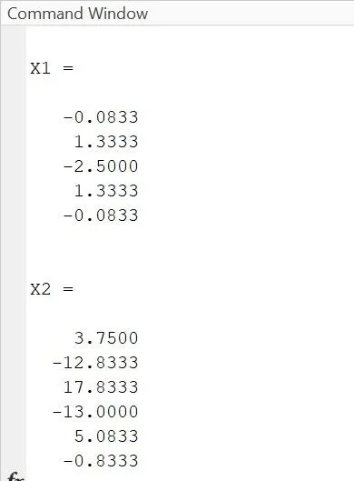
screenshots of matrix co-efficient a,b,c,d,e,f of centered, skewed right sided difference and skewed left sided difference 4th order approximations for 2nd order derivative.
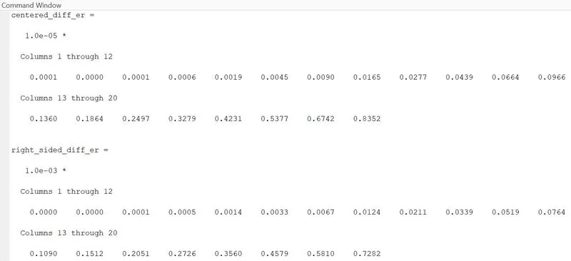
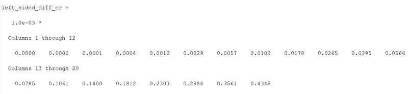
screenshots of numerical calculation errors of centered, skewed right sided difference and skewed left sided difference.
screenshots of plotted graphs:
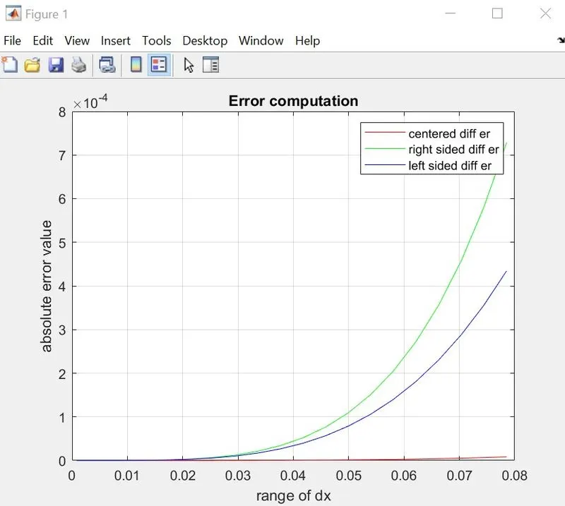
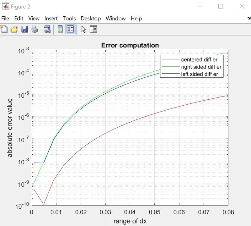
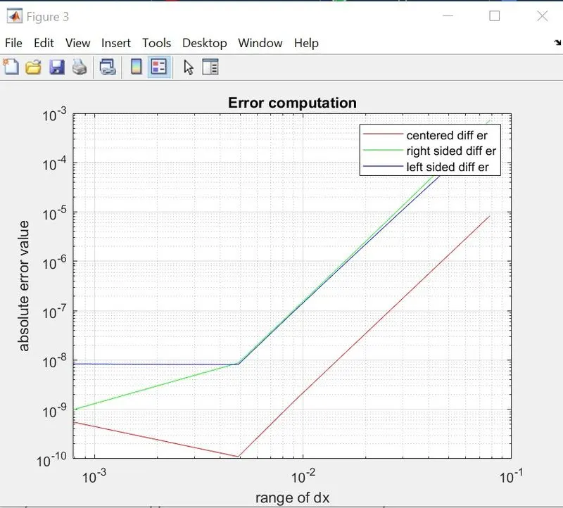
- From the figure 1 we can say centered difference is not clearly visible because of the that type of graph which is a normal plot.
- From the figure 2 we can say it is much clear than the figure 1
- from the figure 3 we can clearly see the graph of all the errors,
- From that we can say that centered difference error is always maintaing a lest error value at all the times.
- But for the symmetric skewed scheme, at some points of right sided difference is higher and at some points left sided difference is higher.
Question:
In your own words, describe why a skewed scheme is useful? What can a skewed scheme do that a CD scheme cannot?
Answer:
skewed scheme is very useful in the cases of nodal points when the nodal points are in the start points and at the end points, in that cases we cannot apply centered scheme, but centered scheme has a advatage where the error value is less compared to other schemes.