Week 4.1 - Genetic Algorithm

Finding the global maxima of stalagmite function

Aim:

• To find the global maxima of stalagmite function
• To optimize using the MATLAB software.

Objectives:

• To explain genetic algorithm in own words and explain the syntax
• To write the code to perform the global maxima and optimization.
• To explain the code in step-wise manner.
• To mention the errors came across the program
• To mention the steps taken to overcome the errors.
• To attach the screenshots related to errors, solutions and outputs.

Genetic algorithm theory:

• Genetic algorithm is the optimization technique. There are so many methods for optimization and GA is one of the methods for optimization.
• This method was actually came from the concept of genetics and natural selection. This theory was proposed by Charles Darwin and the theory is known as “Charles Darwin’s theory of natural evolution”
• The algorithm repeatedly modifies a population of individual solutionsand generates a population of points at each iteration.

Syntax:

x = ga(fun,nvars,A,b,Aeq,beq,lb,ub)

This defines the set of lower and upper bounds on the design variables, x, so that a solution is found in the range 1b x UB.

Governing equations:

f1_x1 = (sin((5.1*3.14*x)+.5))^6;

f1_y1 = (sin((5.1*3.14*y)+.5))^6;

f2_x2 = exp(-4*log(2)*(x-.0667)^2/0.64);

f2_y2 = exp(-4*log(2)*(y-.0667)^2/0.64);

[v] = -(f1_x1*f1_y1*f2_x2*f2_y2);

MATLAB CODE:

PROGRAM CODE:

clear all
close all
clc

% defining our search space
x = linspace(0,0.6,150);
y = linspace(0,0.6,150);

% creating a 2D mesh
[xx yy] = meshgrid(x,y);

% evaluating the stalagmite function
for i = 1:length(xx)
    for j = 1:length(yy)
        input_vector(1) = xx(i,j);
        input_vector(2) = yy(i,j);
        f(i,j) = stalagmite(input_vector);
    end
end


% surfc(xx,yy,f)
shading interp
[x,fval] = ga(@stalagmite,2)
        



x = linspace(0,0.6,150);
y = linspace(0,0.6,150);
num_cases = 50;

% study - 1 - statistical behaviour
for i = 1:num_cases
    [inputs, fopt(i)] = ga(@stalagmite, 2);
    xopt(i) = inputs(1);
    yopt(i) = inputs(2);
end

figure(1)
subplot(2,1,1)
hold on
surfc(x, y, -f)
shading interp
plot3(xopt, yopt, -fopt,'marker','o','markersize',5,'markerfacecolor','r')
title('unbounded inputs')
subplot(2,1,2)
plot(-fopt)
xlabel('iterations')
ylabel('function minimum')

tic
% study 2 - statistical behaviour - with upper and lower bounds
for i = 1:num_cases
    [inputs, fopt(i)] = ga(@stalagmite, 2,[],[],[],[],[0;0],[1;1]);
    xopt(i) = inputs(1);
    yopt(i) = inputs(2);
end
study2_time = toc

figure(2)
subplot(2,1,1)
hold on
surfc(x, y, -f)
shading interp
plot3(xopt, yopt, -fopt,'marker','o','markersize',5,'markerfacecolor','r')
title('bounded inputs')
subplot(2,1,2)
plot(fopt)
xlabel('iterations')
ylabel('function minimum')

% study - 3 increasing GA iterations 
options = optimoptions('ga')
options = optimoptions(options,'populationsize',170);

tic
for i = 1:num_cases
    [inputs, fopt(i)] = ga(@stalagmite, 2,[],[],[],[],[0;0],[0.1;0.1],[],[],options);
    xopt(i) = inputs(1);
    yopt(i) = inputs(2);
end
study3_time = toc

figure(3)
subplot(2,1,1)
hold on
surfc(x,y,f)
shading interp
plot3(xopt, yopt, -fopt,'marker','o','markersize',5,'markerfacecolor','r')
title('bounded inputs')
subplot(2,1,2)
plot(fopt)
xlabel('iterations')
ylabel('function minimum')




FUNCTION CODE:

function[v] = stalagmite(input_vector)
x = input_vector(1);
y = input_vector(2);

f1_x1 = (sin((5.1*3.14*x)+.5))^6;
f1_y1 = (sin((5.1*3.14*y)+.5))^6;
f2_x2 = exp(-4*log(2)*(x-.0667)^2/0.64);
f2_y2 = exp(-4*log(2)*(y-.0667)^2/0.64);
[v] = -(f1_x1*f1_y1*f2_x2*f2_y2);
end

Step-wise code explanation:

Step-1:

The first part of the code is to define the interval by using the LINSPACE command.

Step-2:

The second part of the code is to define the two inputs x and y and to create array of x and y values by utilizing the MESHGRID command.

Step-3:

The third part of the code is to evaluate the stalagmite function by using for-end loop, here we input these two values x and y into genetic algorithm.

Step-4:

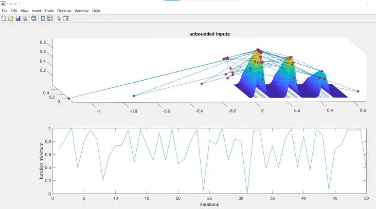
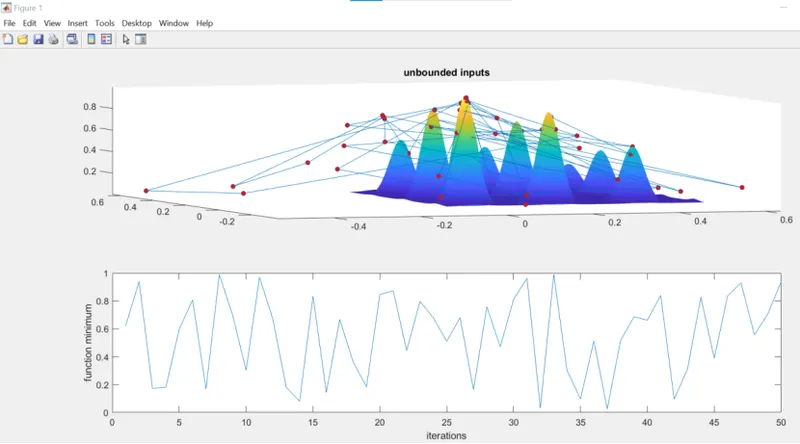
To optimize or improve the genetic algorithm, here we use three cases. Case number one is programmed in a way where the GA doesn’t know the upper and the lower limit by taking all the possible values into consideration which are also called unbounded values and to make the plot.

Step-5:

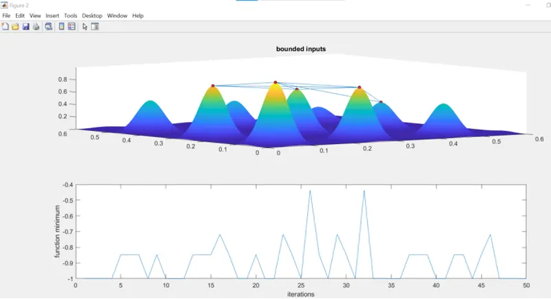
The next part of the code is case 2, here the upper and lower bound values are given and to make the plot.

Step-6:

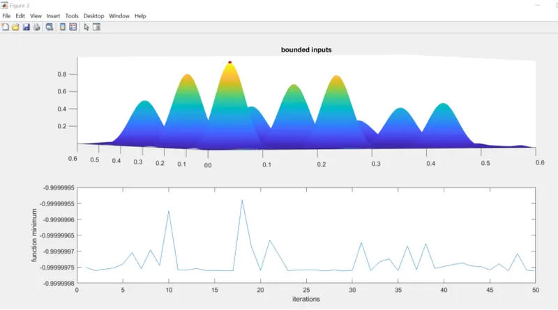
The next part of the code is to generate a plot of global maxima of one value by increasing GA iterations, where it is finely optimized.

Error encountered:

f1_x1 = (sin((5.1*3.14*x)+.5))^6;

f1_y1 = (sin((5.1*3.14*x)+.5))^6;

Instead of y I have typed x again so the error encountered, finally the error is rectified and it is shown in the output.

Output results:

Case1: unbounded inputs

Case-2: bounded inputs

Case-3: single global maxima

Conclusion:

• Explanation of genetic algorithm in own words and syntax is done.
• Code to perform the global maxima and optimization is done.
• Explanation of the code in step-wise manner is done.
• Highlighting the errors came across the program is done.
• Steps taken to overcome the errors is done
• Attachment of screenshots related to errors, solutions and outputs is done.