Week 5.1 - Mid term project - Solving the steady and unsteady 2D heat conduction problem
WEEK 5.1 MID TERM PROJECT : 2 - D STEADY AND UNSTEADY HEAT CONDUCTION EQUATION
AIM:
To solve 2 - d steady and unsteady heat conduction equation by using explicit and implicit methods by the given conditions.
To plot the graphs for steady and unsteady heat conduction equation.
GIVEN:
Top Boundary = 600 K
Bottom Boundary = 900 K
Left Boundary = 400 K
Right Boundary = 800 K
Absolute error criteria is 1e-4
THEORY:
Explicit and implicit method:
These approaches used in numerical analysis for obtaining numerical approximations to the solutions of time-dependent ordinary and partial differential equation as is required in computer simulations of physical processes. Explicit methods calculate the state of a system at a later time from the state of the system at the current time, while implicit method find a solution by solving an equation involving both the current state of the system and the later one.
IMPLICIT METHOD - ITERATIVE SOLVERS:
`A ** X = B`
`A = [L + D + U]`
`[ L + D + U] ** X = B`
`A = [[0, 0, 0], [a21, 0, 0], [a31, a32, 0]]` +`[[a11, 0, 0], [0, a22, 0], [0, 0, a33]]` + `[[0, a12, a13], [0, 0, a23], [0, 0, 0]]`
`A = [[a11, a12, a13], [a21, a22, a23], [a31, a32, a33]]`
2 - D STEADY SATE HEAT CONDUCTION EQUATION:
`(del^2T)/(delx^2) + (del^2T)/(dely^2) = 0`
SECOND ORDER CENTRAL DIFFERENCE SCHEME:
`(del^2T)/(delx^2) = (T(i - 1,j) + 2T(i, j) + T(i + 1,j))/(delx^2)`
`(del^2T)/(dely^2) = (T(i, j-1) + 2T(i, j) + T(i, j + 1))/(dely^2)`
1. JACOBI METHOD:
`[ L + D + U] ** X = B`
`(D ** X)^(K +1) = -(L + U) ** (X)^(K) + B`
`X^(K + 1) = -D^(-1)(L + U)**X^(K) + D^(-1) ** B`
so, `P = -D^(-1)**(L + U)` and Q = `D^(-1)**B`
`X^(K + 1) = PX^(K) + Q`
`X1^(K + 1) = 1/(a11)[b1 - a12**X2^k - a13**X3^k]`
`X2^(K + 1) = 1/(a22)[b2 - a21**X1^k - a23**X3^k]`
`X3^(K + 1) = 1/(a33)[b3 - a31**X1^k - a32**X2^k]`
`T(i,j) = [ (T(i - 1,j) + T(i + 1, j))/(K**delx^2) + (T(i, j-1) + T(i,j+1))/(K**dely^2)]^(old)`
`K = (2 **(delx^2 + dely^2))/(delx^2**dely^2`
2. GAUSS SEIDEL METHOD:
`[L + D + U] ** X = -U**X + B`
`[D + L]**X^(K + 1) = -U**X^K + B`
`X^(K + 1) = -(D + L)^(-1)**U**X^(K) + (D + L)^(-1)**B`
so, `P = -(D + L)^(-1)**U` , `Q = (D + L)^(-1)**B`
`X^(K + 1) = PX^(K) + Q`
`X1^(K + 1) = 1/(a11)[b1 - a12**X2^k - a13**X3^k]`
`X2^(K + 1) = 1/(a22)[b2 - a21**X1^(k + 1) - a23**X3^(k + 1)]`
`X3^(K + 1) = 1/(a33)[b3 - a31**X1^(k + 1) - a32**X2^(k + 1)]`
`T(i,j) = (T(i - 1,j) + T(i + 1, j)^(old))/(K**delx^2) + (T(i, j-1) + T(i,j+1)^(old))/(K**dely^2)`
`K = (2 **(delx^2 + dely^2))/(delx^2**dely^2`
3. SUCCESSIVE OVER RELAXATION (SOR) METHOD:
`[ L + D + U] ** X = B`
`[L + alphaD - alphaD + D + U]**X = B`
`omega ** alpha = 1`
`[L + alphaD]X = [(alpha - 1)D - U]X + B`
`[omegaL + D]X = [ (1 - omega)D - omegaU]X + omegaB`
`X^(k + 1) = (D + omegaL)^(-1) [(1 - omega)D - omegaU]X^K + (D + omegaL)^(-1) omegaB`
so, `P = (D + omegaL)^(-1) [(1 - omega)D - omegaU]` and `Q = (D + omegaL)^(-1) omegaB`
`T(i,j) = (1-omega)T(i,j)^(old) + omega[(T(i - 1,j) + T(i + 1, j)^(old))/(K**delx^2) + (T(i, j-1) + T(i,j+1)^(old))/(K**dely^2)]`
`K = (2 **(delx^2 + dely^2))/(delx^2**dely^2`
2 - D UNSTEADY HEAT EQUATION:
`alpha((del^2T)/(delx^2) + (del^2T)/(dely^2)) = 0`
1.EXPLICIT METHOD:
`T(i,j)^n = (1 - 2K1-2K2)**T(i,j)^(n-1) + K1**[T(i-1,j) + T(i+1,j)]^(n-1)+ k2**[T(i,j-1) + T(i,j+1)]^(n-1)`
`K1 = alpha*(d^2t)/(dx^2)`
`K2 = alpha*(d^2t)/(dy^2)`
IMPLICIT METOD:
`Term_1 = 1/(1 + 2K_1 + 2K_2)`
`Term_2 = k1**Term_1`
`Term_3 = k_2**Term_1`
1. JACOBI METHOD:
`T(i,j)^n = Term_1**T(i,j)^(n-1)+Term_2**[T(i-1,j) + T(i+1,j)]^(old) + Term_3**[T(i,j-1) + T(i,j+1)]^(old)`
2. GAUSS SEIDEL METHOD:
`T(i,j)^n = Term_1**T(i,j)^(n-1) + Term_2[T(i-1,j)+T(i+1,j)^(old)] + Term_3**[T(i,j-1) + T(i,j+1)^(old)]`
3. SUCCESSIVE OVER RELAXATION METHOD:
`T(i,j)^n = (1-omega)**T(i,j)^(old)+omega[Term_1**T(i,j)^(n-1) + Term_2[T(i-1,j)+T(i+1,j)^(old)] + Term_3**[T(i,j-1) + T(i,j+1)^(old)]]`
PROGRAM CODE FOR 2D STEADY HEAT CONDUCTION EQUATION (IMPLICIT):
% 2 - D steady state heat conduction eaquation
close all
clear
clc

% input
L = 1;

% grid points
nx = 150;
ny = nx;

% interval
x = linspace(0, L, nx);
dx = x(2) - x(1);

y = linspace(0, L, nx);
dy = dx;

% initialising the temperature for all cells
T = 300 * ones(nx, ny);

% assining boundary conditions
T(1,:)     = 600;
T(end,:)   = 900;
T(:,1)     = 400;
T(:,end)   = 800;
Told   = T;

% to solve any one of the three cases at a time
iterative_solver  = 3;

% error value
error = 9e9;

% tolerance error value
tol = 1e-4;

% jacobi method
jacobi_iter = 1;
if iterative_solver ==1

    % to calculate the simulation time
    tic

    % to execute the when the loop is greater than the mentioned value
    while(error > tol)

        % space loop
        for i = 2:nx-1
            for j = 2:ny - 1

                % K =  (2*dx^2 + 2*dy^2)/(dx^2 * dy^2)
                % separating the equation into two parts to avoid complexity
                A =  (Told(i-1, j) + Told(i+1, j));
                B =  (Told(i, j-1) + Told(i, j+1));
                T(i,j) =  0.25 * (A + B);
            end
        end

        % to find the maximum of all numbers
        error = max(max(abs(Told - T)));

        % to update te values
        Told = T;
        jacobi_iter = jacobi_iter + 1;
        time_counter = toc;

    end

    figure(1)
    % to flip the reversed plot
    contourf(x, fliplr(y), T, 'ShowText','on')
    pause(0.03)
    colorbar
    xlabel('X - AXIS')
    ylabel('T')
    title(sprintf('Method : JACOBI \n Iteration = %d \n Computation Time = %0.4f S',
           jacobi_iter, time_counter));

end

% gauss seidal method
GS_iter = 1;
if iterative_solver ==2
    tic

    while(error > tol)
        for i = 2:nx - 1
            for j = 2:ny - 1
                A =  (T(i-1, j) + Told(i+1, j));
                B =  (T(i, j-1) + Told(i, j+1));
                T(i,j) =  0.25 * (A + B);
            end
        end

        error = max(max(abs(Told - T)));
        Told = T;
        GS_iter = GS_iter + 1;
        time_counter = toc;
    end


    figure(2)
    contourf(x, fliplr(y), T, 'ShowText','on')
    pause(0.03)
    colorbar
    xlabel('X - AXIS')
    ylabel('T')
    title(sprintf('Method : GAUSS SEIDEL \n Iteration = %d \n Computation Time = %0.4f
          S', GS_iter, time_counter));
end


% successive over relaxation (SOR) method
omega = 1.7;
SOR_iter = 1;
if iterative_solver ==3

    tic
    while(error > tol)
        for i = 2:nx - 1
            for j = 2:ny - 1
                A =  (T(i-1, j) + Told(i+1, j));
                B =  (T(i, j-1) + Told(i, j+1));
                T(i,j) =  (Told(i,j) * (1 - omega)) + (omega * 0.25 * (A + B));
            end
        end

        error = max(max(abs(Told - T)));
        Told = T;
        SOR_iter = SOR_iter + 1;
        time_counter = toc;

    end

    figure(3)
    contourf(x, fliplr(y), T, 'ShowText','on')
    colorbar
    pause(0.03)
    xlabel('X - AXIS')
    ylabel('T')
    title(sprintf('Method : SOR \n Iteration = %d \n Computation Time = %0.4f S',
          SOR_iter, time_counter));
end
STEP - WISE CODE EXPLANATION:
Step - 1:
Give the domain length and number of grid points.
Step - 2:
Specify the interval by using the ‘’LINSPACE’’ command in x and y direction.
Step - 3:
Initialize the temperature for inner nodal cells.
Step - 4:
Assign the given boundary conditions for the domain.
Step - 5:
Mention the error and the tolerance values.
Step - 6:
Use the tic - toc command to calculate the computation time, where tic is placed at the starting of the loop and toc is placed at the end of the loop.
Step - 7:
Use the while loop to make the solution if the error value is greater than the tolerance value.
Step - 8:
To create the space loop for grid points in x and y directions.
Step - 9:
Write the equation to calculate the problem which can be split into two equations in order to avoid complexity and confusion while writing in the MATLAB.
Step - 10:
We need to find the error, where we need to take the maximum error value.
Step - 11:
To plot the graph for each methods.
Step - 12:
To use the contour command to create the plot and to use the flip command to reverse the upside down graph.
Step - 13:
To print the title and to give the legend.
Step - 14:
To print the computation time and number of iterations.
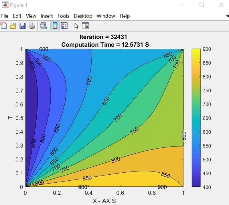
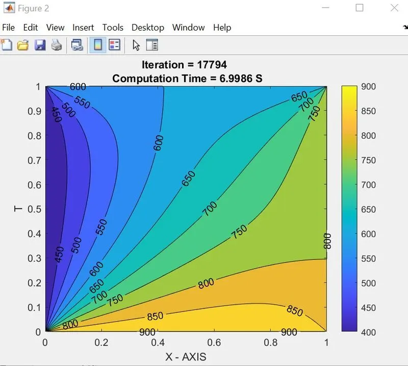
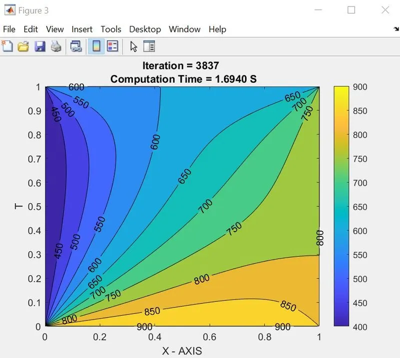
RESULTS AND OUTPUT:
PROGRAM CODE FOR 2D UNSTEADY HEAT CONDUCTION EQUATION (EXPLICIT):
% 2d un-steady heat conduction equation (transient analysis explicit method)
close all
clear
clc

% inputs
L = 1;

% grid points
nx = 50;
ny = nx;

% interval
x = linspace(0, L, nx);
dx = x(2) - x(1);

y = linspace(0, L, nx);
dy = dx;

alpha = 0.0001;
dt = 1;

% initialising the temperature for all cells
T = 300 * ones(nx, ny);

% assining boundary conditions
T(1,:)     = 600;
T(end,:)   = 900;
T(:,1)     = 400;
T(:,end)   = 800;
Told   = T;

CFL_NUMBER = (alpha * dt) * ((1/dx^2) + (1/dy^2));

k1 = alpha * (dt/dx^2);
k2 = alpha * (dt/dy^2);

% calculation of temperature distribution by unsteady (transient) explicit method
term_1 = (1 + (2 * k1) + (2 * k2))^-1;
term_2 = k1 * term_1;
term_3 = k2 * term_1;

tic
counter = 1;
for k = 1 : 5000

    %   explicit iteration scheme
    for i = 2:nx-1
        for j = 2:ny - 1

            % separating the equation into two parts to avoid complexity
            A =  (Told(i-1, j) + Told(i+1, j));
            B =  (Told(i, j-1) + Told(i, j+1));
            T(i,j) = (Told(i,j) * term_1) + (A * term_2) + (B * term_3);
        end
    end

    % to update the values
    Told = T;
    counter = counter +1;
    time_counter = toc;


end
 % plot
    figure(4)
    % to flip the reversed plot
    contourf(x, fliplr(y), T, 'ShowText','on')
    pause(0.03)
    colorbar
    xlabel('XX')
    ylabel('YY')
    title(sprintf(' Method : EXPLICIT \n Iteration = %d \n Computation Time = %0.4f',
          counter - 1, time_counter));
CODE EXPLANATION:
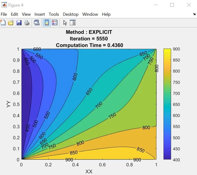
The above mentioned steps are same for 2 - d unsteady heat conduction for explicit and implicit methods, but the only change is to add a time step loop since it is transient where the temperature changes with respect to time.
RESULTS AND OUTPUT:
PROGRAM CODE FOR 2D UNSTEADY HEAT CONDUCTION EQUATION (IMPLICIT):
% 2d un-steady heat conduction equation (transient analysis implicit method)
close all
clear
clc

% inputs
L = 1;

% grid points
nx = 200;
ny = nx;

% interval
x = linspace(0, L, nx);
dx = x(2) - x(1);

y = linspace(0, L, nx);
dy = dx;

alpha = 0.0001;
omega = 1.4;
dt = 1;

% tolerance error value
tol = 1e-4;

% initialising the temperature for all cells
T = 300 * ones(nx, ny);

% assigning boundary conditions
T(1,:)     = 600;
T(end,:)   = 900;
T(:,1)     = 400;
T(:,end)   = 800;
Told   = T;
T_prev_dt = T;
CFL_NUMBER = (alpha * dt) * ((1/dx^2) + (1/dy^2));

k1 = alpha * (dt/dx^2);
k2 = alpha * (dt/dy^2);

% calculation of temperature distribution by unsteady (transient) explicit method
term_1 = (1 + (2 * k1) + (2 * k2))^-1;
term_2 = k1 * term_1;
term_3 = k2 * term_1;

tic
counter = 1;
iterative_solver = 3;

% jacobi method
if iterative_solver == 1

    for k = 1 : 100

        % error value
        error = 9e9;

        while(error > tol)
            % explicit iteration sceme
            for i = 2:nx-1
                for j = 2:ny - 1


                    %separating the equation into two parts to avoid complexity
                    A =  (Told(i-1, j) + Told(i+1, j));
                    B =  (Told(i, j-1) + Told(i, j+1));
                    T(i,j) = (T_prev_dt(i,j) * term_1) + (A * term_2) + (B * term_3);
                end
            end

            error = max(max(abs(Told-T)));

            % to update the values
            Told = T;
            T_prev_dt = T;
            counter = counter + 1;
        end
        time_counter = toc;


    end
    % plot
    figure(5)

    % to flip the reversed plot
    contourf(x, fliplr(y), T, 'ShowText','on')
    pause(0.03)
    colorbar
    xlabel('X - AXIS')
    ylabel('T')
    title(sprintf('2 - D UNSTEADY HEAT CONDUCTION \n Method: JACOBI \n Number of
           Iterations : %d \n Computation Time: %0.4f S', counter - 1, time_counter))
end


% gauss seidal method
if iterative_solver == 2

    for k = 1 : 100

        %
        error = 9e9;

        while(error > tol)
            %   explicit iteration scheme
            for i = 2:nx-1
                for j = 2:ny - 1


                    %separating the equation into two parts to avoid complexity
                    A =  (T(i-1, j) + Told(i+1, j));
                    B =  (T(i, j-1) + Told(i, j+1));
                    T(i,j) = (T_prev_dt(i,j) * term_1) + (A * term_2) + (B * term_3);
                end
            end

            error = max(max(abs(Told-T)));

            % to update the values
            Told = T;
            T_prev_dt = T;
            counter = counter + 1;
        end
        time_counter = toc;


    end

    % plot
    figure(6)
    % to flip the reversed plot
    contourf(x, fliplr(y), T, 'ShowText','on')
    pause(0.03)
    colorbar
    xlabel('X - AXIS')
    ylabel('T')
    title(sprintf('2 - D UNSTEADY HEAT CONDUCTION \n Method: GAUSS SEIDAL \n Number of
          Iterations : %d \n Computation Time: %0.4f S', counter - 1, time_counter))

end

% SOR method
if iterative_solver == 3

    for k = 1 : 100

        %
        error = 9e9;

        while(error > tol)
            %   explicit iteration sceme
            for i = 2:nx-1
                for j = 2:ny - 1


                    % separating the equation into two parts to avoid complexity
                    A =  (T(i-1, j) + Told(i+1, j));
                    B =  (T(i, j-1) + Told(i, j+1));
                    T(i,j) = (1 - omega) * (Told(i,j)) +(omega * ((T_prev_dt(i,j) * term_1) + (A * term_2) + (B * term_3)));
                end
            end

            error = max(max(abs(Told-T)));
            % to update the values
            Told = T;
            T_prev_dt = T;
            counter = counter + 1;
        end
        time_counter = toc;

    end
    % plot
    figure(7)
    % to flip the reversed plot
    contourf(x, fliplr(y), T, 'ShowText','on')
    pause(0.03)
    colorbar
    xlabel('X - AXIS')
    ylabel('T')
    title(sprintf('2 - D UNSTEADY HEAT CONDUCTION \n Method: SOR \n Number of
           Iterations : %d \n Computation Time: %0.4f S', counter - 1, time_counter))

end
RESULTS AND OUTPUT:
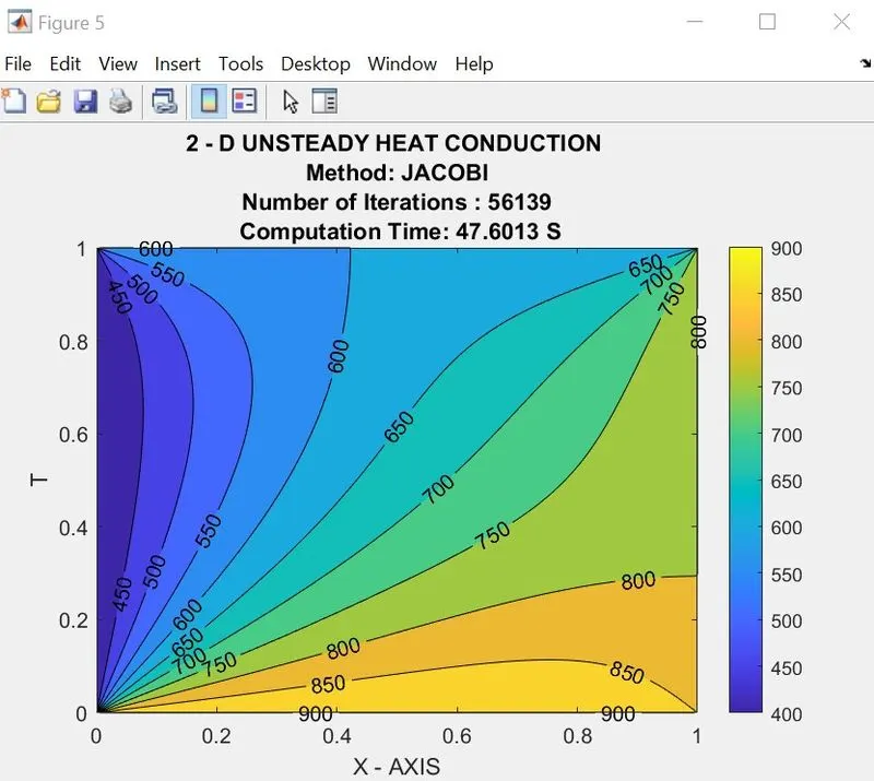
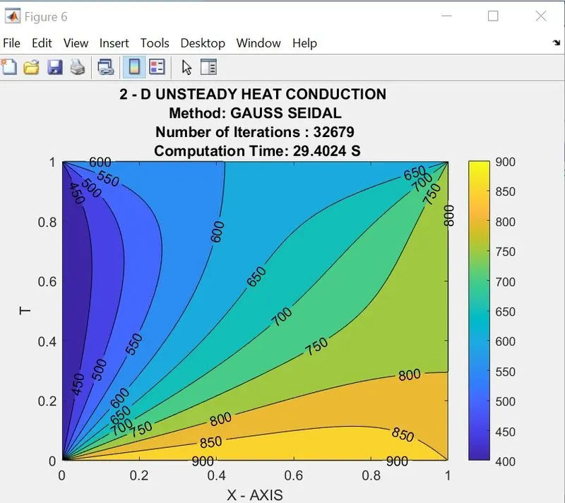
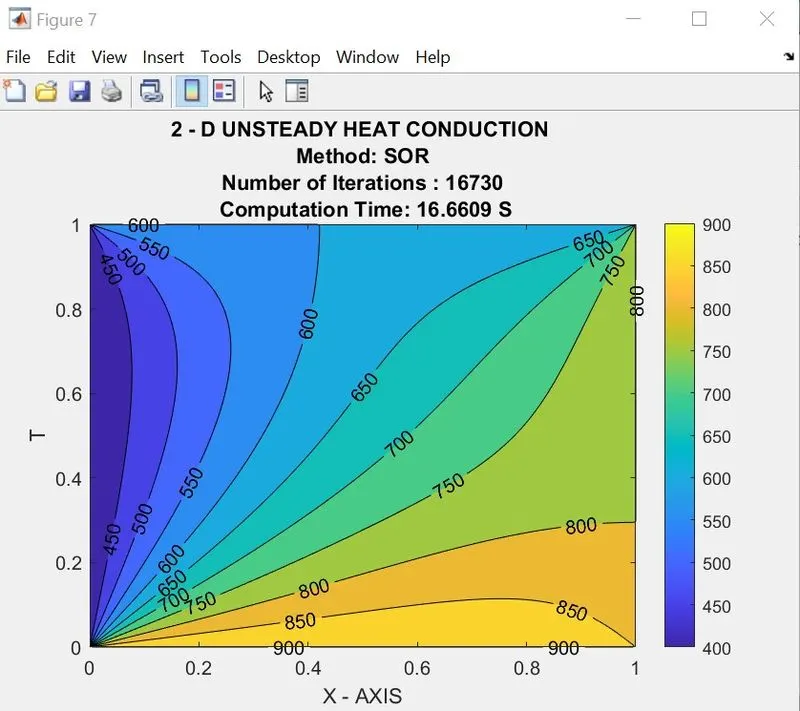
CONCLUSION:
- From the iterations and computation time we can say that SOR method takes very less number of iterations so it takes less time to converge for steady and unsteady 2 - d conduction problem.
- The next quick method for the calculation is Gauss Seidel method.
- Basic theory and explanation of methods is done.
- The graphs are plotted for all the methods.