Week 9 - FVM Literature Review

Finite Volume Method(FVM)

The finite volume method (FVM) is a method for representing and evaluating partial differential equations in the form of algebraic equations. In the finite volume method, volume integrals in a partial differential equation that contain a divergence term are converted to surface integrals, using the divergence theorem. These terms are then evaluated as fluxes at the surfaces of each finite volume. Because the flux entering a given volume is identical to that leaving the adjacent volume, these methods are conservative. Another advantage of the finite volume method is that it is easily formulated to allow for unstructured meshes. The method is used in many computational fluid dynamics packages. "Finite volume" refers to the small volume surrounding each node point on a mesh.

The major differences between FDM & FVM

Finite volume methods can be compared and contrasted with the finite difference methods, which approximate derivatives using nodal values, or finite element methods, which create local approximations of a solution using local data, and construct a global approximation by stitching them together. In contrast a finite volume method evaluates exact expressions for the average value of the solution over some volume, and uses this data to construct approximations of the solution within cells

Need for interpolation schemes and flux limiters in FVM.

In FVM we need to calculate the variables at location other than computational nodes, so it becomes necessary to use interpolation schemes.

It is observed that for convective flow problem interpolation schemes gives good results but in case of shock flow problem we can see long jumps through discountinuities, so in that case we need flux limiter to ascertain these values.

An example:1D linear heat conduction equation

Here we are taking 1D steady state heat conduction equation and descritizing it using FVM

`del/(delx)(alpha(delT)/(delx))+S=0`

S= Source Term responsible for heat generation

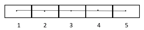
Here points are centers of control volumes

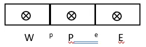
Here there is a control volume P and left and right voulmes are denoted by W and E. The face which connects these voulmes ae are calling it as 'w' and 'e'.

We need Intergral form of governing equation.So as the equation is valid at whole volume so we will integrate the equation for whole volume.

`intdel/(delx)(alpha(delT)/(delx))dV+intSdV=0`

Here dV = Adx

`intdel/(delx)(alpha(delT)/(delx))Adx+intSdV=0`

`(alphaA(delT)/(delx))_w^e+barSdV=0`

where `barSdV=intSdV`

`alpha_eA((delT)/(delx))_e+alpha_wA((delT)/(delx))_w+barSdV=0`

Now to find temperature gradients we need aproximations

`alpha_eA((T_E-T_P)/(Deltax))+alpha_wA((T_P-T_W)/(Deltax))+barSdV=0`

This is conservation equations in FVM form which is heat flux out-heat flux in+source term =0

Here, to find alpha we use interpolation schemes