A MATLAB program to fit the curve of Cp vs Temperature data & find goodness of the curve
Here we are going to fit the curve of the given data of temp v/s Cp in three different ways:
1. Fitting the curve linearly and with cubic polynomial
2. Fitting the curve with the help of splitting the data and fitting linearly
3. Fitting the curve linearly and with cubic polynomial with the help of MATLAB curvefitting toolbox
1. Fitting the curve linearly and with cubic polynomial
Here we are fitting the curve by extracting the polynomial co-efficients and then using them to predict new Cp. Then comparing the new Cp with old Cp to find error and goodness of the curve
Below is the MATLAB code with explanations in the form of comments
clc
clear
close all

cp_data=load('data'); % Load the data file & store in new variable
temp=cp_data(:,1); % Extract the columns to new variable
Cp=cp_data(:,2); % Extract the data

co_eff_1=polyfit(temp,Cp,1); % fitting the curve linearly & finding constants
predicted_cp_1=polyval(co_eff_1,temp); % finding the new data set with new polynomial

co_eff_3=polyfit(temp,Cp,3); % fitting the curve with cubic polynomial & finding constants
predicted_cp_3=polyval(co_eff_3,temp); % finding the new data set with new polynomial

plot(temp,Cp,'linewidth',3,'color','green') %plotting original data set

hold on % Avoiding figure rewrite
plot(temp,predicted_cp_1,'linewidth',3,'color','yellow') %plotting new linear data set
plot(temp,predicted_cp_3,'linewidth',3,'color','red') %plotting new polynomial data set
xlabel('Temperature [K]'); %Labeling X-Axis
ylabel('Specific Heat Cp [KJ/kg-K]'); %Labeling Y-Axis
title('Temp v/s Cp') %Labeling Title
legend('Original Data Set','Linear Fit','Cubic Polynomial Fit') %Diffrentiating Curves
axis([0 3500 900 1500]) %Ranging the axis


% Finding the goodness of the fit
% Initiating values to zero
SSR=0;
SSE=0;
sum=0;
n=length(temp);

% Finding Mean of the Cp data
for i=1:n
    sum=sum+Cp(i);
end

Mean=sum/n;


for i=1:n

    Error = predicted_cp_3(i)-Cp(i);    % Finding Error
    esq=Error^2;                        % Squaring Error to remove -ve sign
    SSE=SSE+esq;                        % SSE = Sum of Square of Error

    Error2= predicted_cp_3(i)-Mean;     % Finding Error from Mean
    esq2=Error2^2;                      % Squaring Error to remove -ve sign
    SSR=SSR+esq2;                       % SSR = Sum of Square of Regression
end

RMSE=sqrt(SSE/n);                       % RMSE = Root Mean Square Error

SST=SSR+SSE;                            % SST = Total of SSE & SSR
RSQUARE=SSR/SST;                        % R-Square

k=1; %Independent Variables
ADJRSQUARE = 1-(((1-RSQUARE)*(n-1))/(n-k-1)); % Adjacent R-Square

%OUTPUT
SSE
RSQUARE
ADJRSQUARE
RMSE
OUTPUT:
SSE =9.4272e+04
RSQUARE =0.9967
ADJRSQUARE =0.9967
RMSE =5.4277
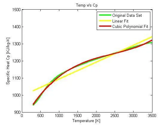
As we can see that the cubic fit is perfect fit while the linear fit is not perfect so as the degree of the polynomial increases the fit becomes more accurate.
2. Fitting the curve with the help of splitting the data and fitting linearly
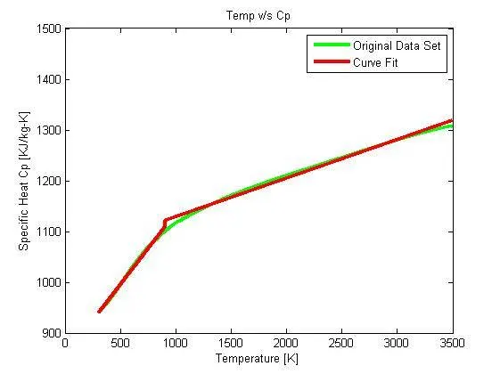
By viewing the curve we found that there is a curvature at 904 K so we splitted the data in two parts and fitted the curve linearly and we found better results than in single linear fit.
clc
clear
close all

cp_data=load('data'); % Load the data file & store in new variable
temp=cp_data(:,1); % Extract the columns to new variable
Cp=cp_data(:,2); % Extract the data

temp1=cp_data(1:604,1); % Extract the columns to new variable
Cp1=cp_data(1:604,2); % Extract the data

temp2=cp_data(605:3200,1); % Extract the columns to new variable
Cp2=cp_data(605:3200,2); % Extract the data

co_eff1=polyfit(temp1,Cp1,1); % fitting the curve upto
predicted_cp1=polyval(co_eff1,temp1);

co_eff2=polyfit(temp2,Cp2,1); % fitting the curve upto
predicted_cp2=polyval(co_eff2,temp2);


for i=1:length(temp)

    if i<605
        predicted_cp(i)=predicted_cp1(i);
    else
        predicted_cp(i)=predicted_cp2(i-604);

    end
end


plot(temp,Cp,'linewidth',3,'color','green')
hold on
plot(temp,predicted_cp,'linewidth',3,'color','red')
xlabel('Temperature [K]');
ylabel('Specific Heat Cp [KJ/kg-K]');
title('Temp v/s Cp')
legend('Original Data Set','Curve Fit')
axis([0 3500 900 1500])

% Finding the goodness of the fit
% Initiating values to zero
SSR=0;
SSE=0;
sum=0;
n=length(temp);

% Finding Mean of the Cp data
for i=1:n
    sum=sum+Cp(i);
end

Mean=sum/n;


for i=1:n

    Error = predicted_cp(i)-Cp(i);    % Finding Error
    esq=Error^2;                        % Squaring Error to remove -ve sign
    SSE=SSE+esq;                        % SSE = Sum of Square of Error

    Error2= predicted_cp(i)-Mean;     % Finding Error from Mean
    esq2=Error2^2;                      % Squaring Error to remove -ve sign
    SSR=SSR+esq2;                       % SSR = Sum of Square of Regression
end

RMSE=sqrt(SSE/n);                       % RMSE = Root Mean Square Error

SST=SSR+SSE;                            % SST = Total of SSE & SSR
RSQUARE=SSR/SST;                        % R-Square

k=1; %Independent Variables
ADJRSQUARE = 1-(((1-RSQUARE)*(n-1))/(n-k-1)); % Adjacent R-Square

%OUTPUT
SSE
RSQUARE
ADJRSQUARE
RMSE
OUTPUT:
SSE =8.1616e+04
RSQUARE =0.9972
ADJRSQUARE =0.9972
RMSE =5.0503
3. Fitting the curve linearly and with cubic polynomial with the help of MATLAB curvefitting toolbox
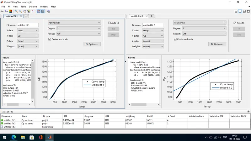
So, Here we are using the curve fitting toolbox to improve the cubic polynomial by normalizing the curve and using te option center and scale
clc
clear
close all

cp_data=load('data');
temp=cp_data(:,1);
Cp=cp_data(:,2);


hold on
[f1,gof1]=fit(temp,Cp,'poly1','Normalize','on')
plot(f1,temp,Cp)
[f3,gof3]=fit(temp,Cp,'poly3','Normalize','on')
plot(f3,temp,Cp)


xlabel('Temperature [K]');
ylabel('Specific Heat Cp [KJ/kg-K]');
title('Temp v/s Cp')
legend('Original Data Set','Linear Fit','Cubic Polynomial Fit')
OUTPUT:
f1 =
Linear model Poly1:
f1(x) = p1*x + p2
where x is normalized by mean 1900 and std 923.9
Coefficients (with 95% confidence bounds):
p1 = 91.24 (90.34, 92.14)
p2 = 1183 (1182, 1184)
gof1 =
sse: 2.1630e+06
rsquare: 0.9249
dfe: 3198
adjrsquare: 0.9249
rmse: 26.0072
f3 =
Linear model Poly3:
f3(x) = p1*x^3 + p2*x^2 + p3*x + p4
where x is normalized by mean 1900 and std 923.9
Coefficients (with 95% confidence bounds):
p1 = 15.03 (14.79, 15.27)
p2 = -25.19 (-25.4, -24.98)
p3 = 64.19 (63.72, 64.66)
p4 = 1208 (1208, 1208)
gof3 =
sse: 9.4272e+04
rsquare: 0.9967
dfe: 3196
adjrsquare: 0.9967
rmse: 5.4311
Questions with Answers
Q1. How to make a curve fit perfectly?
A1 To get the perfect fit either you can increase the order of polynomial & check the goodness of the fit with various parameter
Q2. How to get the best fit?
Note: Best fit and perfect fit are two completely different phenomena.
A2 To get the best fit we need to find the fit in which error is minimum.
Q3. What could be done to improve the cubic fit?
A3 To improve the cubic fit you need to normalize the fit or Center and scale the fit in Curve Fitting ToolBox
REFRENCES:
MATLAB HELP