A MATLAB code to find the global maxima of the stalagmite function

INTRODUCTION:

STALAGMITE

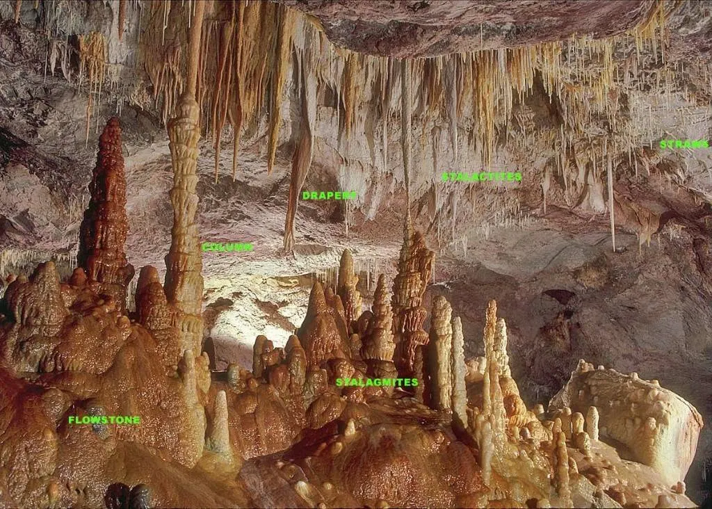
A stalagmite is a type of rock formation that rises from the floor of a cave due to the accumulation of material deposited on the floor from ceiling drippings. Stalagmites are typically composed of calcium carbonate, but may consist of lava, mud, peat, pitch, sand, sinter and amberat. [1]

STALAGMITE FUNCTION:

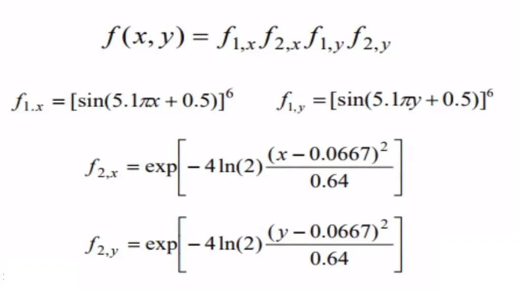
function f=stalagmite(input_vector)

x=input_vector(1);
y=input_vector(2);

f1x=sin(5.1*pi*x+0.5)^6;
f1y=sin(5.1*pi*y+0.5)^6;

f2x=exp((-4*log(2))*((x-0.0667)^2)/(0.64));
f2y=exp((-4*log(2))*((y-0.0667)^2)/(0.64));

f=f1x*f1y*f2x*f2y;
f=-f;
end

Here at the end the function is reversed with a negative sign because ga only minimizes the function and we want to find global maxima.

As stalagmate function has many peaks but we want to find maximum peak.

This function has many local maxima but we are interested in global maxima.

Genetic Algorithm (GA):

Nature has always been a great source of inspiration to all mankind. Genetic Algorithms (GAs) are search based algorithms based on the concepts of natural selection and genetics. GAs are a subset of a much larger branch of computation known as Evolutionary Computation.

GAs were developed by John Holland and his students and colleagues at the University of Michigan, most notably David E. Goldberg and has since been tried on various optimization problems with a high degree of success.

In GAs, we have a pool or a population of possible solutions to the given problem. These solutions then undergo recombination and mutation (like in natural genetics), producing new children, and the process is repeated over various generations. Each individual (or candidate solution) is assigned a fitness value (based on its objective function value) and the fitter individuals are given a higher chance to mate and yield more “fitter” individuals. This is in line with the Darwinian Theory of “Survival of the Fittest”.

In this way we keep “evolving” better individuals or solutions over generations, till we reach a stopping criterion.

Genetic Algorithms are sufficiently randomized in nature, but they perform much better than random local search (in which we just try various random solutions, keeping track of the best so far), as they exploit historical information as well.[2]

SYNTAX FOR GA :

[x,fval,exitflag,output,population,scores] = ga(fun,nvars,A,b,Aeq,beq,lb,ub,nonlcon,options)

Input Arguments

fun – Objective Function

nvars,- No. of Variables

A – Linear Inequality constraints (real matrix)

b - Linear Inequality constraints (real vector)

Aeq - Linear equality constraints (real matrix)

beq - Linear equality constraints (real vector)

lb – Lower Bounds

ub – Upper Bounds

nonlcon – Nonlinear constraints

options – Optimization options

Output Arguments

x – Solution

fval – Objective function value at solution

exitflag – Reason ga stopped

output – Information about optimization process

population – Final population

scores – Final scores [3]

MATLAB CODE TO FIND THE GLOBAL MAXIMA

This code is explained with the help of comments

clc
clear
close all

x=linspace(0,0.6,150);  % Input Array for xx
y=linspace(0,0.6,150);  % Input Array for yy
num_cases=50;           % Number of cases
[xx, yy]=meshgrid(x,y); % Create a 2-D grid with uniformly spaced x-coordinates and y-coordinates


for i=1:length(xx)
    for j=1:length(yy)
        input_vector(1)=xx(i,j);    % Takes the input from the grid
        input_vector(2)=yy(i,j);    % Takes the input from the grid
        f(i,j)=stalagmite(input_vector);    % Processing the inputs through stalagmite function and storing the output
    end
end


% Increasing the population size to converge to the result
options = optimoptions('ga','PopulationSize', 300);

 tic % Start stopwatch timer
for i=1:num_cases
    % ga takes minimum two inputs first function & second variable
    % ga can also take other inputs such as constraints, bounds, etc.
    
    [outputs, fopt(i)]=ga(@stalagmite,2,[],[],[],[],[0;0],[1;1],[],[],options);
    % outputs = ga predicts the minimum optimum solution
    % fopt = Objective function value at the solution
    xopt(i)=outputs(1); % storing the optmum value for each case
    yopt(i)=outputs(2); 
end
study_time=toc %Read elapsed time from stopwatch

figure(1)

%subplot(m,n,p) divides the current figure into an m-by-n grid and creates axes in the position specified by p. 
subplot(2,1,1)
hold on
surfc(x,y,f) %Contour plot under surface plot
shading interp % Set color shading 

% 3-D point or line plot collapse
% To visualize how algorithm is performing
plot3(xopt,yopt,fopt,'marker','o','markersize',5,'markerfacecolor','r') 
title('bounded inputs')

% Plotting the optimum results obtained
subplot(2,1,2)
plot(fopt)
xlabel('Iterations')
ylabel('Function Minimum')

%output
outputs

OUTPUT:

study_time = 26.6316

outputs = 0.0668 0.0668

This are the co-ordinates of the global maxima and above is the time taken to run the study

So, below is the three studies which required to investigate the problem and to reach the final solution.

STUDY 1- STATISTICAL BEHAVIOUR

We are storing the optimum values of ga and plotting the ouputs which ga predicts as a output values

we also introduces tic toc function to find how long it take to perform the study.

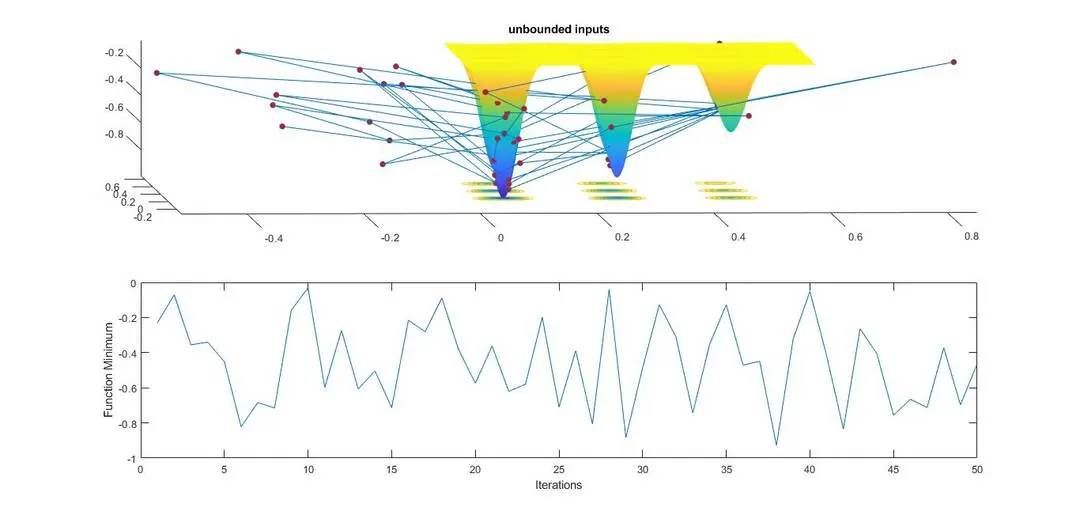
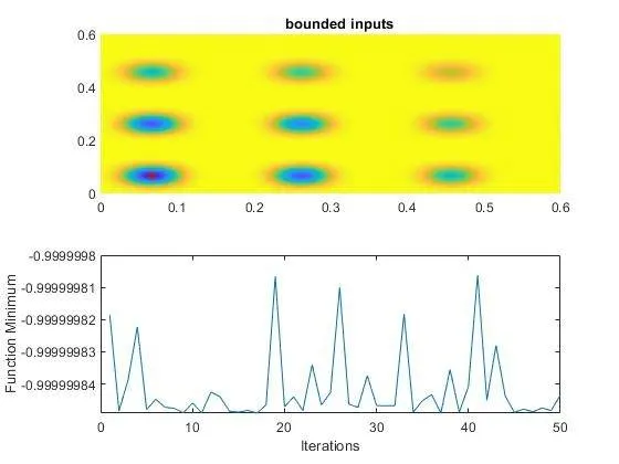
So, below now we can see the graph with the help of plot3 command we got the optimum values which ga predicts.

So, from this graph we came to know that the function is operating outside the bounds where the objective function doesnot exist so we moved to study -2

STUDY 2- statistical behaviour with upper and lower bounds

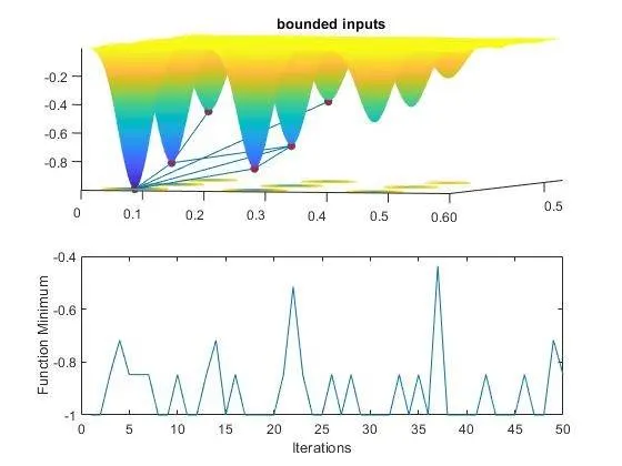
So, the findings from the study-1 is applied in this study by giving upper and lower bounds to the ga and we found that the optimum solution has converged to few solutions, but still the solution is not unique it keeps on changing so to solve this limitations we have to increase the population size of the ga.

STUDY 3- STATISTICAL BEHAVIOUR WITH BOUNDS & INCREASED POPULATION SIZE

So, in this study we have increased the population size using the option input argument of ga.

This will help in greater probalility of reaching the fittest solution i.e. optimum minimum solution.

Errors occured

Error using optimoptions Invalid solver specified. Provide a solver name or handle (such as 'fmincon' or @fminunc). Type DOC OPTIMOPTIONS for a list of solvers.

Solved : By using LATEST VERSION OF MATLAB 2020b having GLOBAL OPTIMIZATION TOOLBOX

It will not work in MATLAB Online as there is no option to insert toolbox online

REFERENCES:

[1] Stalagmite - Wikipedia

[2] Genetic Algorithms - Introduction - Tutorialspoint

[3] MATLAB HELP: doc ga