An MATLAB program to plot PV diagram of an Air standard otto Cycle

An ideal otto cycle consists of the following processes

1-2 Isentropic Compression

The piston moves from BDC to TDC, the gas volume decreases, and the pressure increases because work is done on the gas by the piston.

2-3 Isochoric Heat Addition

The beginning of the combustion of the fuel/air mixture. The combustion occurs very quickly and the volume remains constant. Heat is released during combustion which increases both the temperature and the pressure

3-4 Isenropic Expansion

The piston moves from BDC to TDC, the volume in increased, and the pressure falls as work is done by the gas on the piston.

4-1 Isochoric Heat Rejection

The exhaust valve is opened and the residual heat in the gas is exchanged with the surroundings. The volume remains constant and the pressure adjusts back to atmospheric conditions.

The following Image has been taken as a reference to understand the otto cycle from NASA website

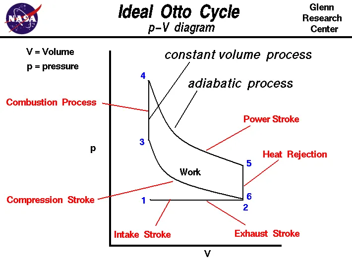
We are going to produce such diagram with the help of MATLAB

by using the thermodynamic co-relations for various processes.

The MATLAB Code is explained below with the help of comments:

% A Program to simulate PV diagram of otto cycle
clc
clear
% 1-2 Isentropic Compression
% 2-3 Isochoric Heat Addition
% 3-4 Isenropic Expansion
% 4-1 Isochoric Heat Rejection

% Inputs 
P1=101325; %Pressure at state 1
T1=500;    %Temperature at state 1
gamma=1.4; %Adiabatic Index
T3=2300;    % %Temperature at state 3
% Engine Geometric Parameters
d=0.1; % Bore Diameter
l=0.1; % Stroke Length
r=12;  % Compression Ratio

Vs=(pi/4)*d^2*l;    %Swept Volume/Stroke Volume
syms Vc;    % Denoting Symbol to Vc=Clearance Volume
Vc=solve(r==(Vc+Vs)/Vc,Vc); % Solving for Vc
Vc=double(Vc); % Converting from symbol to double data type

V1=Vs+Vc; %Volume at state 1
% State 2
V2=Vc; %Volume at state 2 

syms P2; % Denoting Symbol
P2=solve(P1*V1^gamma==P2*V2^gamma,P2); % Solving for P2 by adiabatic eqn
P2=double(P2); % Converting from symbol to double data type

syms T2; % Denoting Symbol
T2=solve(P1*V1/T1==P2*V2/T2,T2); % Solving for T2 by Ideal gas equation
T2=double(T2); % Converting from symbol to double data type

% State 3
V3=V2;

syms P3; % Denoting Symbol
P3=solve(P3*V3/T3==P2*V2/T2,P3); % Solving for P3 Ideal gas equation
P3=double(P3); % Converting from symbol to double data type

% State 4
V4=V1; %Volume at state 4

syms P4; % Denoting Symbol
P4=solve(P3*V3^gamma==P4*V4^gamma,P4); % Solving for P4 by adiabatic eqn
P4=double(P4); % Converting from symbol to double data type


lcr=0.15; % Connecting rod length 
a=l/2; %crank pin radius = stroke length / 2
R=lcr/a; % Connecting rod length/crank pin radius
theta=0:180; % Angle


c12=P1*V1^gamma;
% Relation between Volume and angle in adiabatc process
Ve=(1+0.5*(r-1)*(R+1-cosd(theta)-(R.^2-sind(theta).^2).^0.5))*Vc;
Pe=c12./Ve.^gamma;

c34=P3*V3^gamma;
theta=180:360;

% Relation between Volume and angle in adiabatc process
V=(1+0.5*(r-1)*(R+1-cosd(theta)-(R.^2-sind(theta).^2).^0.5))*Vc;
P=c34./V.^gamma;


plot(Ve,Pe,V,P,[V2 V3],[P2 P3],[V4 V1],[P4 P1])
xlabel('Volume')
ylabel('Pressure')
title('Otto Cycle')

Efficiency=1-1/(r^(gamma-1))

OUTPUT:

Efficiency =

0.6299

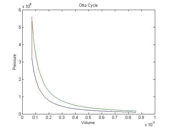
The above PV diagram of otto cycle represents all the 4 processes from state 1 to 4

& the efficiency of the above cycle is 62.3%

The emiprical relation between angle and volume during the adiabatic process helped in creating the above diagram.

Errors Faced:

1. Inputs must be a scalar and a square matrix.
To compute elementwise POWER, use POWER (.^) instead.

BEFORE : Pe=c12/Ve^gamma;

AFTER : Pe=c12./Ve.^gamma;