A MATLAB program that will simulate the pendulum motion.

In this project we are going to program the ode funtion of the pendulum and find the displacement and velocity with the help of ode45 function.

After getting the results of the displacement we will use it in the for loop to create simulation of pendulum.

STEPS:

1. First we will define the data given in the question

2. Create a ODE function file that we can use in the program

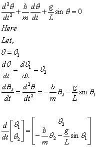
In this step we will convert the following 2nd order ode into equation

Inserting the function file

function [dtheta_dt]=ode_func(t,theta,b,g,l,m)

theta1=theta(1);
theta2=theta(2);
dtheta1_dt=theta2;
dtheta2_dt=-(b/m)*theta2-(g/l)*sin(theta1);
dtheta_dt=[dtheta1_dt ;dtheta2_dt];

end

3. Using ode45 function to find the derivatives of the above variables

ode45 takes three input
1 Function
2 Integration limits i.e. time span
3 Initial Conditions i.e x0,xdot0

Syntax

[time, output]=ode45(Function, time span, [xo xdot0]);

4. Plotting Graphs

1 Displacement v/s Time

2 Velocity v/s Time

5. Creating Animation and Video file

For this we used for loop denoted two points A & B

whose coordinates are A(0,0) fixed to the wall and for

B(0-length*cos(displcaement) 0-length*sin(displcaement) )

Now, Inserting the MATLAB code explained line by line with the help of MATLAB code

clc
clear
close all

m=1;  % m = mass of the ball in kg,
b=0.05; % b=damping coefficient.
l=1;    % L = length of the pendulum in m,
g=9.81;  % g = Gravitational Acceleration in m/s2,

fr=1; %frames

%theta=[Displacement Velocity]
% Initial Conditions
theta_0=[0 3]; %{Initial Displacement & Initial Velocity}

%time
t_span=0:0.1:20;
%ode45 takes three input
%1. Function
%2. Integration limits i.e. time span
%3. Initial Conditions i.e x0,xdot0
[t, theta]=ode45(@(t,theta) ode_func(t,theta,b,g,l,m),t_span,theta_0);


figure(1) % Helps in creating multple graphs
hold on %Helps to prevent the overwrite the previous graph
plot(t,theta(:,1),'red') %plots the displacement in 1st column
plot(t,theta(:,2),'green') %plots the velocity in 2nd column
axis([0 10 -5 5]) % denotes the axis range
legend('Displacement','Velocity') % Diffrentiate the graphs with the help of legend
xlabel('Time') % Labeling the X-axis
ylabel('Values') % Labeling the Y-axis
title('x./t') % Title

displacement=theta(:,1)';

for i=displacement
    
    % Let define the co-orinate points of the Pendulum
    A=[0 0]; % Denotes the fixed point of the Pendulum
    B=[A(1)-l*cos(i) A(2)-1*sin(i)]; % Denotes the End Point of the Pendulum where the mass is attached
    figure(2) % Helps in creating multple graphs
    plot([10.02 9.98],[10,10],[A(2) B(2)], [A(1) B(1)],'-o','linewidth',2,'MarkerSize',10,'MarkerEdgeColor','g')
    axis([-2 2 -2 2 ]) % Denotes the axis span
    pause(0.001) % pausing the iteration
    
     M(fr)=getframe(gcf); %M denotes movie with fr frames
                             %getframe will form gcf=current figure handle
        fr=fr+1; % fr=No. of frames, intiated as fr=1
    
end



movie(M) % binding frames into movie
videofile=VideoWriter('pendulum.avi','Uncompressed AVI'); %Creating video file
open(videofile)  % opening the video file
writeVideo(videofile,M)% writing the video file
close(videofile) % closing the video file

OUTPUT:

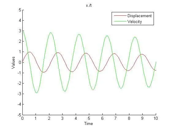
The output video file represents the motion of the pendulum up to 20 sec with the help of the displacement values which obtained from solving ode equations.

Errors occured while coding:

Error 1: Undefined function or variable 'Displacement'.

Before: legend(Displacement,Velocity)

After: legend('Displacement','Velocity')

Error 2: overwrite the previous graph

Before:

After: hold on