Week 9 - FVM Literature Review

there are total 4 numerical methods

1) Finite Element Method(FEM)

2)Boundary Element Method(BEM)

3)Finite Volume Method (FVM)

4)Finite Difference Method(FDM)

FVM

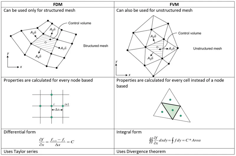
The finite-volume method is similar to the finite differencing method in that the CAD model is divided into very small but finite sized elements of geometrically simple shapes .apart from this, the finite volume method is very different from the finite differencing method, beginning with the concept of elements, which are instead reffed to as a cell.

A finite volume method discretization is based upon an integral form of the PDE to be solved and can handle discontinuities in solutions.PDE is written in from which can solve for a given finite volume. the computational domain is discretized into finite volume and then for every volume the governing equation of the conserved variable and thus calculation of fluxes is very important in FVM.

the finite volume method strength is that it only needs to do flux evaluation for the cell boundaries. This also holds for nonlinear problems. which makes it extra powerful for robust handling of conservation laws appearing in transport problems.

the local accuracy of the finite-volume methods, such as close to the corner of interest can be increased by refining the mesh around that corner, however, the function that approximate the solution when using the finite volume method cannot be easily made of higher-order this is a disadvantage of the finite volume method compared to the finite-difference method.

The basic advantage of this method over FDM is it does not require the use of structured grids and the effort to convert the given mesh into a structured numerical grid internally is completely avoided, as with FDM the resulting approximate solution is discrete but the variables are typically placed at cell-centered finite volume methods, in nay case, the value of field variables at nonstorage lov=ction are obtained using interpolation

Interpolation schemes

the approximations of surface and volume in integrals require values of the variable at a location other than the computational nodes of the control volume, values at these locations are obtained using interpolation formulate.

`del/(delx)muphi=del/(dx)(Gamma(delphi)/(delx))`

phi is out solution variable (scalar)

mu is velocity

`amma is diffusion cofficien`

1)upwind interpolation scheme

this scheme takes into account the direction of fluid flow and based on it a value of the solution variable at the face is approximated by its value at the upstream computational node

.for example, if the fluid moved left to right

2)liner interpolation scheme

in order to approximate the value variable at the control volume face center by two nearest computational nodes locations. this is equivalent to the center difference scheme first orders derivative .it is second orders accurate and produces an oscillatory solution. the relation for linear interpolation gave below.

flux limiter

for convective fluid flow .it is the observer that low order schemes are usually stable but quite dissipation in nature around the points of discontinuity or socks while higher orders scheme are unstable in nature and show oscillation in the vicinity of discontinuity or shocks highly accurate and oscillation scheme are known as high resolution scheme