Week 7 - Simulation of a 1D Super-sonic nozzle flow simulation using Macormack Method
non-conservation forms
clear all
close all
clc

%inputs
n=31
x=linspace(0,3,n)
dx=x(2)-x(1)
gamma=1.4
%cfl=max((v+sqrt(t))*dt/dx)

%calculate intial profiles
rho=1-0.316*x;
t=1-0.2314*x; % t=temprature
v=(0.1+1.09*x).*t.^0.5;
%cfl=max((v+sqrt(t))*dt/dx)

%area
a=1+2.2*(x-1.5).^2;
%time stpes
nt=1000
dt=0.001;
%outer time loop
for k=1:nt
    rho_old=rho;
    v_old=v;
    t_old=t;
    %predictor method

    %continos equstion
     for j=2:n-1
         dvdx=(v(j+1)-v(j))/dx;
         drhodx=(rho(j+1)-rho(j))/dx;
         dtdx=(t(j+1)-t(j))/dx;
         dlogadx=(log(a(j+1))-log(a(j)))/dx;
          %continos equstion
         drhodt_p(j)=-rho(j)*dvdx-rho(j)*v(j)*dlogadx-v(j)*drhodx;
         %momentum equstion
         dvdt_p(j)=-v(j)*dvdx-(1/gamma)*(dtdx+(t(j)/rho(j))*drhodx);
         %enery eustion
         dtdt_p(j)=-v(j)*dtdx -(gamma-1)*t(j)*(dvdx+v(j)*dlogadx);

          %solustion update
          rho(j)= rho(j)+ drhodt_p(j)*dt;
          v(j)=v(j)+dvdt_p(j)*dt;
          t(j)=t(j)+dtdt_p(j)*dt;
     end
     %corretor method
     for j=2:n-1
         dvdx=(v(j)-v(j-1))/dx;
         drhodx=(rho(j)-rho(j-1))/dx;
         dtdx=(t(j)-t(j-1))/dx;
         dlogadx=(log(a(j))-log(a(j-1)))/dx;
          %continos equstion
         drhodt_c(j)=-rho(j)*dvdx-rho(j)*v(j)*dlogadx-v(j)*drhodx;
         %momentum equstion
         dvdt_c(j)=-v(j)*dvdx-(1/gamma)*(dtdx+(t(j)/rho(j))*drhodx);
         %enery eustion
         dtdt_c(j)=-v(j)*dtdx -(gamma-1)*t(j)*(dvdx+v(j)*dlogadx);


     end
    %compute the average time derivateve
    drhodt=0.5*(drhodt_p+drhodt_c);
    dvdt=0.5*(dvdt_p+dvdt_c);
    dtdt=0.5*(dvdt_p+dtdt_c);
    %final solustion update
    for i=2:n-1
    rho(i)=rho_old(i)+drhodt(i)*dt;
     v(i)=v_old(i)+dvdt(i)*dt;
     t(i)=t_old(i)+dtdt(i)*dt;
    end
% apply the boundary condoction
v(1)=2*v(2)-v(3); %inlet
v(n)=2*v(n-1)-v(n-2);
rho(n)=2*rho(n-1)-rho(n-2);
t(n)=2*t(n-1)-t(n-2);
%pressure
p=rho.*t;
%mach num
M=v./sqrt(t);
%mass flow rate
m=rho.*a.*v;
figure(3)
if k==1
    plot(x,m)
    hold on
end
if k==50
    plot(x,m)
end
if k==250
    plot(x,m)
end
if k==750
    plot(x,m)
end
if k==1400
    plot(x,m)
end

end
xlabel('nozzle length')
ylabel('mass flow rate')
legend('1adt','50dt','250dt','750dt','1400dt')
title('variation of mass flow rate at diffrent time steps')
figure(1)
subplot(5,1,1)
plot(x,v)
xlabel('nozzle length')
ylabel('velocity')
subplot(5,1,2)
plot(x,rho)
xlabel('nozzle length')
ylabel('dencity')
subplot(5,1,3)
plot(x,t)
xlabel('nozzle length')
ylabel('temprature')
subplot(5,1,4)
plot(x,p)
xlabel('nozzle length')
ylabel('pressure')
subplot(5,1,5)
plot(x,M)
xlabel('nozzle length')
ylabel('mach num')
figure(2)
plot(x,m)
xlabel('nozzle length')
ylabel('mass flow rate') 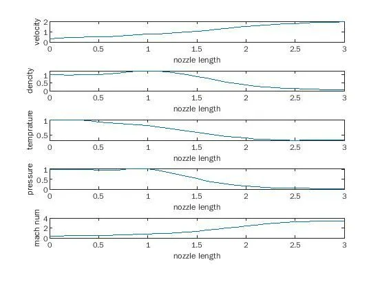
Steady-state distribution of primitive variables inside the nozzle
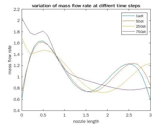
Time-wise variation of the primitive variables
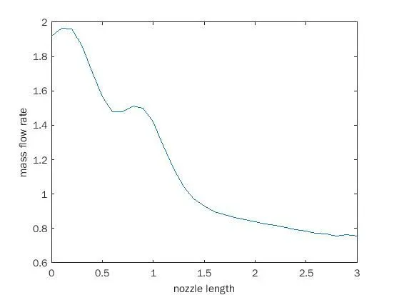
flow rate distribution inside the nozzle at different time steps during the time-marching process
conservation forms
clear all
close all
clc

%inputs
n=31
x=linspace(0,3,n)
dx=x(2)-x(1);
gamma=1.4
%cfl=max((v+sqrt(t))*dt/dx)

%calculate intial profiles
% rho=1-0.316*x;
% t=1-0.2314*x; % t=temprature
% v=(0.1+1.09*x).*t.^0.5;
% %cfl=max((v+sqrt(t))*dt/dx)
for i=1:n
    if x(i)<=0.5
    rho(i)=1;
    t(i)=1;
    end
    if x(i)>0.5  && x(i)<=1.5
    rho(i)=1-0.366*(x(i)-0.4);
    t(i)=1-0.167*(x(i)-0.5);
    end
    if x(i)>1.5
    rho(i)=0.634-0.3879*(x(i)-1.5);
    t(i)=0.833-0.3507*(x(i)-1.5);
    end


end
%time stpes
nt=1000
dt=0.001;
gamma=1.4;
%area
a=1+2.2*(x-1.5).^2;

v=0.59./(rho.*a);
U1=rho.*a;
U2=rho.*a.*v;
U3=U1.*(t/(gamma-1)+(gamma/2)*v.^2);
F1=U2;
F2=U2.^2./U1+(gamma-1)/(gamma)*(U3-(gamma/2)*(U2.^2./U1));
F3=gamma*U2.*U3./U1-0.5*gamma*(gamma-1)*(U2.^3./U1.^2);


%outer time loop
for k=1:nt
    U1_old=U1;
    U2_old=U2;
    U3_old=U3;
    %predictor method

    %continos equstion
     for j=2:n-1
%          dvdx=(v(j+1)-v(j))/dx;
%          drhodx=(rho(j+1)-rho(j))/dx;
%          dtdx=(t(j+1)-t(j))/dx;
%          dlogadx=(log(a(j+1))-log(a(j)))/dx;
          %continos equstion
         dU1dt_p(j)=-(F1(j+1)-F1(j))/dx;
         J2=(1/gamma)*rho(j)*t(j)*(a(j+1)-a(j))/dx;
         %momentum equstion
         dU2dt_p(j)=-(F2(j+1)-F2(j))/dx+J2;
         %enery eustion
         dU3dt_p(j)=-(F3(j+1)-F3(j))/dx;
          %solustion update
         U1(j)= U1(j)+ dU1dt_p(j)*dt;
          U2(j)=U2(j)+dU2dt_p(j)*dt;
          U3(j)=U3(j)+dU3dt_p(j)*dt;

     end
     %predicor update


          rho=U1./a;
          t=(gamma-1)*(U3./U1-(gamma/2)*(U2./U1).^2);
F1=U2;
F2=U2.^2./U1+(gamma-1)/(gamma)*(U3-(gamma/2)*(U2.^2./U1));
F3=gamma*U2.*U3./U1-0.5*gamma*(gamma-1)*(U2.^3./U1.^2);

     %corretor method

         %continos equstion
     for j=2:n-1
%          dvdx=(v(j+1)-v(j))/dx;
%          drhodx=(rho(j+1)-rho(j))/dx;
%          dtdx=(t(j+1)-t(j))/dx;
%          dlogadx=(log(a(j+1))-log(a(j)))/dx;
          %continos equstion
         dU1dt_c(j)=-(F1(j)-F1(j-1))/dx;
         J2=(1/gamma)*rho(j)*t(j)*(a(j)-a(j-1))/dx;
         %momentum equstion
         dU2dt_c(j)=-(F2(j)-F2(j-1))/dx+J2;
         %enery eustion
         dU3dt_c(j)=-(F3(j)-F3(j-1))/dx;


     end
    %compute the average time derivateve
   dU1dt=0.5*(dU1dt_p+dU1dt_c);
    dU2dt=0.5*(dU2dt_p+dU2dt_c);
    dU3dt=0.5*(dU3dt_p+dU3dt_c);
    %final solustion update
    for i=2:n-1
    U1(i)=U1_old(i)+dU1dt(i)*dt;
     U2(i)=U2_old(i)+dU2dt(i)*dt;
     U3(i)=U3_old(i)+dU3dt(i)*dt;
    end
    %final update update
    rho=U1./a;
    t=(gamma-1)*(U3./U1-(gamma/2)*(U2./U1).^2);
    v=U2./U1;
% apply the boundary condoction
U1(1)=a(1);%inlet
U2(1)=2*U2(2)-U2(3);
U3(1)=U1(1)*(t(1)/(gamma-1)+0.5*gamma*v(1)^2);
%outlet
U1(n)=2*U1(n-1)-U1(n-2);
U2(n)=2*U2(n-1)-U2(n-2);
U3(n)=2*U3(n-1)-U3(n-2);
%pressure
p=rho.*t;
%mach num
M=v./sqrt(t);
%mass flow rate
m=rho.*a.*v;
figure(3)
if k==1
    plot(x,m)
    hold on
end
if k==50
    plot(x,m)
end
if k==250
    plot(x,m)
end
if k==750
    plot(x,m)
end
if k==1400
    plot(x,m)
end

end
xlabel('nozzle length')
ylabel('mass flow rate')
legend('1dt','50dt','250dt','750dt','1400dt')
title('variation of mass flow rate at diffrent time steps')
figure(1)
subplot(5,1,1)
plot(x,v)
xlabel('nozzle length')
ylabel('velocity')
subplot(5,1,2)
plot(x,rho)
xlabel('nozzle length')
ylabel('dencity')
subplot(5,1,3)
plot(x,t)
xlabel('nozzle length')
ylabel('temprature')
subplot(5,1,4)
plot(x,p)
xlabel('nozzle length')
ylabel('pressure')
subplot(5,1,5)
plot(x,M)
xlabel('nozzle length')
ylabel('mach num')
figure(2)
plot(x,m)
xlabel('nozzle length')
ylabel('mass flow rate')
figure()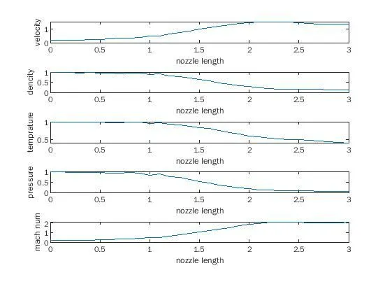
Steady-state distribution of primitive variables inside the nozzle
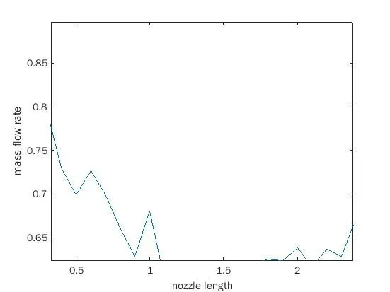
Time-wise variation of the primitive variables
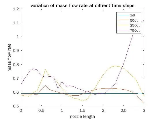
Variation of Mass flow rate distribution inside the nozzle at different time steps during the time-marching process
1)the conservation from yields a better mass flow distribution. the conservation from simply does a better job of conserving mass.
2)the nonconservation from leads to smaller residuals.the amount by which the residuals decay is often used as an index of the quality of the numerical algorithm in this case the nonconservation form does a better job.
3)there is no clear superiority pf either from in terms of accuracy of results. the nonconservation seems to produce slightly more accurate results for the primitive variables and the conservation seems to pressure slightly more accurate results for flux variables. the results, in either case, are certainly satisfactory.
4)comparing the amount of calculation effort to achieve a solution, we note that the solution of the conservation requires marginally more work .most of this is due to the need to decode the primitive variable from flux variable .such decoding is not necessary when you are solving the nonconservation.