Week 3.5 - Deriving 4th order approximation of a 2nd order derivative using Taylor Table method

central differencing

No of nodes =p+q-1

where p is the order of derivative

q is the order of approximation

the number of nodes=2+4-1=5

Taylor table c

dx^2f''(i)	f(i)	f'(i)dx	f''(i)dx^2	f'''(i)dx^3	f''''(i)dx^4
af(i-2)	a	-2a	2a	-(4a/3)	2a/3
bf(i-1)	b	-b	b/2	b/6	b/24
cf(i)	c	0	0	0	0
df(i+1)	d	d	d/2	d/6	0
ef(i+2)	e	2e	2e	4e/3	2e/3
sum of coefficient	0	0	1	0	0

sloveing question

p=[1 1 1 1 1;-2 -1 0 1 2;4/2 1/2 0 1/2 4/2;-8/6 -1/6 0 1/6 8/6;16/24 1/24 0 1/24 16/24]

q=[0;0;1;0;0]

px=q

x=inv p*q

so 'x' we get value as

a=-0.0833;
b=1.3333;
c=-2.5000;
d=1.3333;
e=-0.0833:

Rifgt hand difference schem

No of nodes =p+q

where p is the order of derivative

q is the order of approximation

the number of nodes=2+4=6

Taylor table

dx^2f''(i)	f(i)	f'(i)dx	f''(i)dx^2	f'''(i)dx^3	f''''(i)dx^4	f'''''(i)dx^5
zf(i)	z	0	0	0	0	0
gf(i+1)	g	g	g/2	g/6	g/24	g/120
hf(i+2)	h	2h	4h/2	8h/6	16h/24	32h/120
jf(i+3)	j	3j	9j/2	27j/6	81j/24	243j/120
kf(i+4)	k	4k	16k/2	64k/6	256k/24	1024k/120
lf(i+5)	l	5l	25l/2	126l/6	625l/24	3125l/120
sum cofficients	0	0	1	0	0	0

sloveing question

p=[1 1 1 1 1;0 1 2 3 4 5;0 1/2 4/2 9/2 16/2 25/2;0 1/6 8/6 27/6 64/6 126/6 ;0 1/24 16/24 81/24 256/24 625/24 ; 0 1/120 32/120 243/120 1024/120 3125/120]

q=[0;0;1;0;0]

px=q

x=inv p*q

so 'x' we get value as

z=3.7500
g=-12.8333
h=17.8333
j=-13.0000
k=5.0833
l=0.8333

Left hand difference scheme

No of nodes =p+q

where p is the order of derivative

q is the order of approximation

the number of nodes=2+4=6

Taylor table

dx^2f''(i)	f(i)	f'(i)dx	f''(i)dx^2	f'''(i)dx^3	f''''(i)dx^4	f'''''(i)dx^5
of(i-5)	o	-5o	25o/2	-125o/6	625o/24	-3125o/120
pf(i-4)	p	-4p	16p/2	-64p/6	256p/24	-1024p/120
qf(i-3)	q	-3q	9q/2	-27q/6	81q/24	-243q/120
rf(i-2)	r	-2r	4r/2	-8r/6	16r/24	-32r/120
sf(i-1)	s	-s	s/2	-s/6	s/24	-s/120
tf(i)	t	0	0	0	0	0
sum of coefficient	0	0	1	0	0	0

loveing question

p=[1 1 1 1 1;-5 -4 -3 -2 -1 0; 25/2 16/2 9/2 4/2 1/2 ; 0 -125/6 -64/6 -27/6 -8/6 -1/6 0 ;625/24 256/24 81/24 16/24 1/24 ;-3125/120 -1025/120 -243/120 -32/120 -1/120 0 ]

q=[0;0;1;0;0]

px=q

x=inv p*q

so 'x' we get value as

o=-0.8333
p=5.0833
q=-13.0000
r=17.8333
s=-12.8333
t=3.7500

clear all
close all
clc
%analytical function
x=pi/3;
dx=linspace(pi/10,pi/100,100)
f=@(x)(exp(x)*cos(x));
g=@(x) (-2*exp(x)*sin(x));
d2f=g(x);
func=f(x);
A=[0;0;1;0;0];
%for right skeww differnce schemem
%coeffient_of _taylore _table
%P=[1 1 1 1 1;-2 -1 0 1 2;4/2 1/2 0 1/2 4/2;-8/6 -1/6 0 1/6 8/6;16/24 1/24 0 1/24 16/24]
%centraldiffrence scheme constan value 
a=-0.0833;
b=1.3333;
c=-2.5000;
d=1.3333;
e=-0.0833
%claculatig value and erroe by cenral diffrencing
%difing varible 
central_diff=zeros(1,100);
error_cetral_diff=zeros(1,100)
right_sdiff=zeros(1,100);
err_rigth=zeros(1,100);
left_sdiff=zeros(1,100)
err_left=zeros(1,100);
for i=1:length(dx)
    %calulating value and error by central difference schenme
    a=-0.0833;
    b=1.3333;
    c=-2.5000;
    d=1.3333;
    e=-0.0833

    central_diff(i)=(a*f(x-2*dx(i))+b*f(x-dx(i))+c*f(x)+d*f(x+dx(i))+e*f(x+2*dx(i)))/(dx(i))^2;
    error_cetral_diff(i)=abs(central_diff(i)-d2f)
    %calclating value and error by right diffrernce
    z=3.7500
    g=-12.8333
    h=17.8333
    j=-13.0000
    k=5.0833
    l=0.8333
    %right_sdiff(i)=(z*f(x)+g*f(x+dx(i))+h*f(x+2*dx(i))+j*f(x+3*dx(i))+k*f(x+4*dx(i)+l*f(x+5*dx(i)))/(dx(i))^2
    right_sdiff(i)=(z*f(x)+g*f(x+dx(i))+h*f(x+2*dx(i))+j*f(x+3*dx(i))+k*f(x+4*dx(i)+l*f(x+5*dx(i)))/(dx(i))^2)
    err_rigth(i)=abs(right_sdiff(i)-d2f);
    %calculting value and error by left diffrene
    o=-0.8333
    p=5.0833
    q=-13.0000
    r=17.8333
    s=-12.8333
    t=3.7500
    left_sdiff(i)=(o*f(x-5*dx(i))+p*f(x-4*dx(i))+q*f(x-3*dx(i))+r*f(x-2*dx(i))+s*f(x-dx(i))+t*f(x))/(dx(i))^2;

    err_left(i)=abs(left_sdiff(i)-d2f);
end
 %plotting 
 figure(1)
 loglog(dx,error_cetral_diff,"b")
 hold on
 loglog(dx,err_rigth,"g")
 loglog(dx,err_left,"r")
 xlabel('range_of_dx')
 ylabel('error')
 legend('centraldiff','rigthdiff','liftdiff')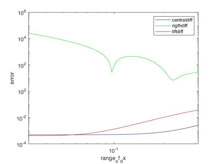

*central differencing scheme better than other two because as per result obtained its showing very less error.

*lift and right side scheme using only one side data so it having more error whereas central scheme use data from both sides so it having less error.

why skewed scheme useful

event though the central difference method uses both side points for some system we will not sufficient data on that case central different e method have no use, in that case, the skew scheme more cone in the picture.

What can a skewed scheme do that a CD scheme cannot Do

CDS cont applied at boundary layer because we will not data lift to right at the time, in such case also skew scheme used.