Week 9 - FVM Literature Review
FINITE VOLUME METHOD(FVM)
Finite volume method(FVM):- The finite volume method is a method for representing and evaluating partial differential equations in form of algebraic equations.
finite volume method discretization is based upon an integral form of the PDE to be solved(eg. conservation of mass, momentum, or energy). The PDE(partial differential equation) is converted into an integral form in terms of volume integral, and then by mathematical operation(by Gauss Divergence theorem) volume integral is converted into surface integrals. The above PDE can be solved for finite volume or cells.
Here the given body or domain to be studied is discretized into finite volumes and then for every volume, the governing equations are solved. The resulting system of equations usually involves fluxes of the conserved variable, and thus the calculation of fluxes is very important in FVM.
FVM method is conservative in nature because of the way it is discretized. Terms are evaluated as fluxes at the surfaces of each finite volume. Because the flux entering a given volume is identical to that leaving the adjacent volume, this method is conservative. In FVM as fluxes are actually solved and fluxes exiting on cell is inlet of the adjacent cell there for it is conservative in nature.
Actually, in FVM a point is considered in every discretized volume of the domain which is basically the center of gravity of that volume, and all the properties or parameters of that particular control volume are stored at this point which is the average value of that parameter of the volume.
let's study the above with example,
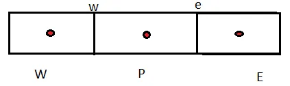
Consider an arbitrary body and divide it into three volumes namely W, P, and E, and the boundary between W and P is named w and between P and E is e.
Here we will try to solve the 1D heat conduction equation within P volume
`del/(delx)(alpha*delT/(delx)) + S =0` ---------------1D heat conduction equation
as the above equaiton is conservative in nature, therefore it is true for even a small volume in the P domain.
Now integrating above eqution for entire volume
`int(del/(delx)(alpha*delT/(delx)) + S)dV =0``.......................volume intetral of the governing equaiton.
`int(del/(delx)(alpha*delT/(delx)))dV + intSdV =0
limits for the integration will be from w to e.
Gauss Divergence Theorem
According to the Gauss Divergence Theorem, the surface integral of a vector field A over a closed surface is equal to the volume integral of the divergence of a vector field A over the volume (V) enclosed by the closed surface.
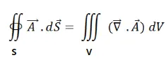
now converting the above equaiton in surface integral by Guss divergence therorem
`int(del/(delx)(alpha*delT/(delx)))Adx + intSdV =0`..............surface integral of 1D heat conduction equation
`[alpha*A*(delT)/(delx)]^eundersetw``+ overlineSdV =0`
`[alpha*A(delT)/(delx)]undersete``- [alpha*A*(delT)/(delx)]undersetw` `+ overlineSdV =0`
`alpha*A[TundersetE``- TundersetP``] - alpha*A[TundersetP``-Tundersetw``] + overlineSdV =0`-----------1
inlet heat flux - outlet heat flux + source term for heat =0
so we can see at the end the conservative nature of equation and in terms of flux.
DIFFERENCE BETWEEN FINITE VOLUME METHOD(FVM) AND FINITE DIFFERENCE METHOD(FDM)
| FINITE DIFFERENCE METHOD(FDM) | FINITE VOLUME METHOD(FDM) |
|
|
INTERPOLATION SCHEMES:-
In finite volume method to evaluate the surface integral of the governing equations in the control volume, it requires values at certain locations(at the boundary face or internal face between two adjacent volumes) other than computational nodes, and the values at these locations are achieved by interpolation schemes.
As we can in the above equation 1 to evaluate the equation in control volume P we need to have values at the faces e and w which are faces between two adjacent faces of control volume P.
Various interpolation schemes are:-
- Upwind interpolation schemes (UIS)
- Liner interpolation schemes
- Quadratic upwind interpolation schemes
- Hybrid
Upwind interpolation schemes
Upwind interpolation/upwind differencing depends on the direction of mass flux
`phi` represents the all the variable of the computational nodes.
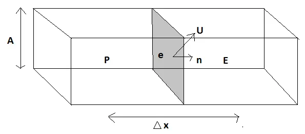
`Fundersete`=`rhoundersete``*Aundersete``*(Uundersete``*hatn)`
`Fundersete`>0 , means mass flow out of the cell
`Fundersete`<0, means mass flow into the cell
the value of
`phiundersete` = `phiundersetP` (`Fundersete` >0, flow out )
`phiundersete` =`phi undersetE``(Fundersete` <0, flow into)
linear interpolation
Approximate the value at the control volume face by linear interpolation of the values of two nearest nodes.
`phiundersete``= psi*phiundersetE``+ (1-psi)phiundersetP`
`psi = (abs(underset(e)(x)-underset(P)(x) ))/abs(underset(E)(x) - underset(P)(x)`
`0<= phi>=1`
second order accurate
but this scheme is unbound
Flux limiter:-
Flux limiter is used in high-resolution schemes described by PDEs.
They are used to avoid the spurious oscillations that would otherwise occur with high order spatial discretization schemes due to shocks, discontinuities or sharp changes in the solution domain.
The use of flux limiter together with an appropriately high-resolution scheme, makes the solution total variation diminishing.
Flux limiters are also called slope limiters because they both have the same mathematical form, and both have the effect of limiting the solution gradient near shocks or discontinuities. In general, the term flux limiter is used when the limiter acts on system fluxes, and slope limiter is used when the limiter acts on system states (like pressure, velocity, etc.).
High-resolution schemes are used in the numerical solution of partial differential equations where high accuracy is required in the presence of shocks or discontinuities. They have the following properties:
- Second- or higher-order spatial accuracy is obtained in smooth parts of the solution.
- Solutions are free from spurious oscillations or wiggles.
- High accuracy is obtained around shocks and discontinuities.
- The number of mesh points containing the wave is small compared with the first-order scheme with similar accuracy.