Week 7 - Simulation of a 1D Super-sonic nozzle flow simulation using Macormack Method
AIM:- To simulate the isentropic flow through a quasi 1D subsonic-supersonic nozzle.
- Need to derive both the conservation and non-conservation forms of the governing equations and solving them using MacCormack's technique.
- Need to determine the steady-state temperature distribution for the flow-field variables and investigate the difference between the two forms of governing equations by comparing their solutions.
Plots to form are:
1. Steady-state distribution of primitive variables inside the nozzle
2. Time-wise variation of the primitive variables
3. Variation of Mass flow rate distribution inside the nozzle at different time steps during the time-marching process
4. Comparison of Normalized mass flow rate distributions of both forms
GIVEN:- Inputs from John D. Anderson book, Part III chapter 7.
Primitive variables are:-
1.Pressure(p) 2.Temperature(T) 3.Density(`rho`) 4.Velocity(V)
We have a Convergent - Divergent nozzle, having a steady and isentropic flow inside it.
Flow at the inlet comes from a reservoir where pressure and temperature are denoted by `punderset0` and `Tunderset0` respectively.
The cross-sectional area of the reservoir is very large (Theoretically,A`rarr infty`) and hence the velocity is very small (V `rarr 0`).
At the exit, flow expands isentropically to supersonic velocity, where exit pressure, temperature, velocity, Mach number are denoted by `pundersete`,`Tundersete`,`Vundersete`,`Mundersete` respectively.
In the convergent section, flow is subsonic, at the throat is sonic and in the divergent section, flow is supersonic.
`poversetast`,`Voversetast`,`Toversetast` and M=1 are pressure, velocity, temperature, and mach no. at the throat.
Area at throat=`A^ast`
speed of sound at throat=`aunderset0`
Subsonic -supersonic isentropic nozzle flow 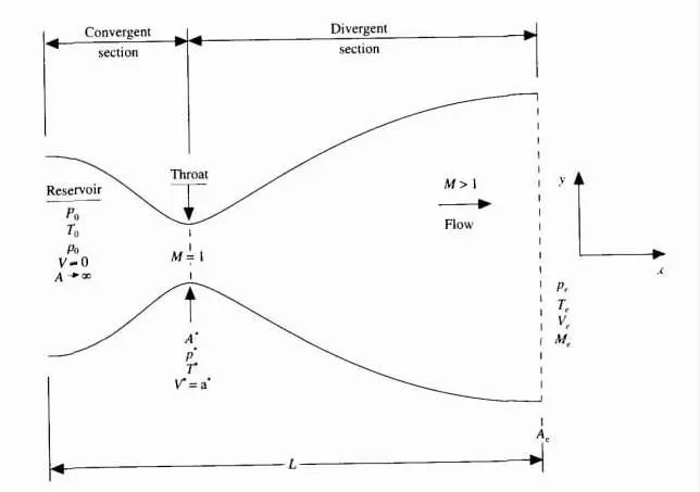
THEORY :-
Quasi one-dimensional nozzle flow:
We are treating the flow inside the nozzle as a one-dimensional flow, that is the flow properties are uniform across cross-section A.
Although the area of the nozzle is changes as a function of distance along that section i.e x-direction. So in reality the flow field is two-dimensional (XY plane), we make the assumption that the flow properties vary only with x. Such flow is defined as quasi-one-dimensional flow.
NON DIMENSIONALIZE FORM OF PARAMETERS
IN our equations we would be using the non dimensionalize equation i.e our parameters would be dimensionless.
X(disatnce of a point from the start of the nozzle)=`x/L`,
area(A)=`A/A^ast`
density=(`rho/(rhounderset0`)
velocity=`V/(aunderset0`
Temperature = `T/(Tunderset0`
Calculation of time step:-
The time step is governed by the system of the analogous equations that provide stability to the solution
`Deltat = C*Deltax/(a+v)`
C=Courant number, for the stability of solution C`<= 0.5`
a=local speed of sound,
in nondimensional form speed of sound is given by, a=`T^(1/2)`
V=local flow velocity at a point in the flow
`Deltat =C*(Deltax)/(T^0.5+V`
As we can see the time step depends on 'a' and 'v' which change in direction of flow so the time step would be different at every node. So time steps should be selected very carefully. In our problem, we would be taking the minimum of all the values of the timestep. So we would have a single timestep for all grid points.
`Deltat=min(Deltat^1 ,Deltat^2 ,Deltat^3,.......,Deltat^n)`
Mass flow rate = `rho*A*V`
Macc no. (M)=`V/T^0.5`
MacCormack method:-
In computational fluid dynamics, the MacCormack method is widely used as a discretization scheme for the numerical solution of hyperbolic partial differential equations. This method is elegant and easy to understand and program.
MacCormack method is a time marching method having a two-step first Predictor step and followed by the second called Corrector step
Predictor step:- The partial differential parameter(eg- `df/dtundersetp`) is evaluated at the n+1 time level by forward differencing. And then the solution is updated(eg.-`foversetast` = `funderseti`+`df/dt*Deltat`).
Corrector step:- Now in this step the solution from the predictor step is corrected of evaluating the above partial differential by backward differecing
(`df^ast/dt`)
the final update will be, `(df/dt )`average = average of predictor and corrector
final solution for second-time step will be `foverset2` = f(initail) + `(df/dt)`average.*dt.
Creating mess
Length of the nozzle (X)=3 unit
`0<=X>=3`
no. of nods(n)=31
Mess size=distance between two consecutive nodes = x(2)-x(1)
Area profile of nozzle(A) = `1+2.2(X-1.5)^2
NON. CONSERVATIVE FORM of Quasi 1-D subsonic - supersonic nozzle
Initial profile
density(`rho')=1-0.3146*X
temperature(T)=1-0.2314*X
velocity(V)=(0.1 + 1.09*X)*`T^0.5`
Governing equation of non-conservative form in non dimensionlize form
Continuity equation
`drho/dt=-rho*dv/dt -rho*v*d(lnA)/dx - v*drho/dx`
Momentum equation
`dv/dt = -v*dv/dx -1/rho(dT/dx + (t/rho)*drho/dx)`
Energy equation
`dT/dx = -v*dT/dx -(gamma -1)*T*(dv/dx + V*d(lnA)/dx)`
Boundary conditions
inlet condition
density`(rho(1))=1`
temperature,T(1)=1
velocity, V(1)=2*V(2)-V(3)
outlet condition
density(`rho(n)`)=`2*rho(n-1) - rho(n-2)`
temperature(T(n))=2*T(n-1) - T(n-2)
velocity(V(n)) = 2*V(n-1) - V(n-2)
CONSERVATIVE FORM of Quasi 1-D subsonic - supersonic nozzle
initial profile
for `0<=x>=0.5`
`rho=1`
`T=1`
for `0.5<=x>=1.5`
`rho=1-0.366(x-0.5)`
`T=1-0.167(x-0.5)`
for `1.5<=x>=3.5`
`rho=0.634-0.3879(x-1.5)`
`T=0.833-0.3507(x-1.5)`
V=`0.59/(rho*A)`
`gamma=1.4`
Governing equation of Conservative form in nondimensional form
Continuity equation
`del(rho*A)/(delt) + del(rho*A*V)/(delx) =0`
Momentum equation
`del(rho*A*V)/(delt) +del[roh*A*V^0.5 + (1/gamma)*p*A]/(delx) = (1/gamma)*p*delA/(delx)`
Energy equation
`del[rho*(e/(gamma-1)+gamma/2*V^2)*A]/(delt) + del[rho(e/(gamma-1)+ gamma/2*V^2)*V*A + p*A*V]/(delx) =0`
U are Solution vector
U1=`rho*A`
U2=`rho*A*V`
U3=`rho*(e/(gamma-1) + gamma/2*V^2)*A`
F are flux vector
`F1=rho*A*V`
F2`=rho*A*V^2 +1/gamma *p*A`
F3=`rho*(e/(gamma-1) + gamma/2*V^2)*V*A + rho*A*V`
J is source vector
`J2 = 1/gamma*p*delA/(delx)`
now our governing equation in terms of U,F,J are
`delU1/(delt) = -del(F1)/(delx)` -------continuity
`del(U2)/(delt) = -del(F2)/(delx) + J2` ------- momentum
`del(U3)/(delt) = -del(F3)/(delx)` -----------energy
Boundary Conditions
inlet condition
U1(1) = A(1)
U2(1)=2*U2(2) - U2(3)
U2(1) =U1(1)*(`T/(gamma-1) + gamma/2*V^2(1)`)
outlet condition
U1(n)=2*U1(n-1) - U1(n-2)
U2(n)=2*U2(n-1) - U2(n-2)
U3(n)=2*U3(n-1) - U3(n-2)
CODING PART:-
In the coding firstly we typed the code separately for both the forms i.e conservative an non-conservative form and genarted all the desired results but for the comparision of normalized or after steady state mass flow rate in between two forms , we just converted the previously typed code into a functional code and call both the function in a sperated code having out as a plot comapring the mass flwo rate between to forms.
d coding for the conservative part:-
clear all
close all
clc
n=31;
x=linspace(0,3,n);
dx=x(2)-x(1);

% nozzle area
a=1+2.2*(x-1.5).^2;
 for j =1:length(x)
     if  x(j)>=0 && x(j)<=0.5
        rho_c(j)=1;
         t_c(j)=1;
     elseif x(j)>=0.5 && x(j)<=1.5
        rho_c(j)=1-0.366*(x(j)-0.5);
         t_c(j)=1-0.167*(x(j)-0.5);
     elseif x(j)>=1.5 && x(j)<=3.5
        rho_c(j) = 0.634-0.3879*(x(j)-1.5);
         t_c(j)=0.833-0.3507*(x(j)-1.5);
     end
  end
 % velocity
  v_c=(0.59)./(rho_c.*a);


gama=1.4;
% definig solution vector
U1=rho_c.*a;
U2=rho_c.*a.*v_c;
U3=rho_c.*(t_c/(gama-1)+(gama/2).*(v_c.^2)).*a;

% pressure
p_c=rho_c.*t_c;


rho=1-0.3146*x; % density
t=1-0.2314*x; %tempreature
v=(0.1 + 1.09*x).*t.^0.5; % velocity
a=1+2.2*(x-1.5).^2; % crossectioinal area

nt=1400;

[mass_flow_rate_c] = cons(n,dx,x,gama,a,rho_c,v_c,t_c);

[mass]=noncons(n,dx,x,a,rho,v,t);


figure(1)
plot(x,mass,'linewidth',2)
hold on
plot(x,mass_flow_rate_c,'linewidth',2)
title('comparision of mass flow rate ')
xlabel('x(lenth of nozzle)')
ylabel('mass flow rate')
legend('non-conservative','conservative')
function for the conservative form
function [mass_flow_rate_c,rho_c,v_c,t_c] =cons(n,dx,x,gama,a,rho_c,v_c,t_c)
n=31;
x=linspace(0,3,n);
dx=x(2)-x(1);

% nozzle area
a=1+2.2*(x-1.5).^2;
% intial condition
  % rho=density
  %t=temperature
  for j =1:length(x)
     if  x(j)>=0 && x(j)<=0.5
        rho_c(j)=1;
         t_c(j)=1;
     elseif x(j)>=0.5 && x(j)<=1.5
        rho_c(j)=1-0.366*(x(j)-0.5);
         t_c(j)=1-0.167*(x(j)-0.5);
     elseif x(j)>=1.5 && x(j)<=3.5
        rho_c(j) = 0.634-0.3879*(x(j)-1.5);
         t_c(j)=0.833-0.3507*(x(j)-1.5);
     end
  end
 % velocity
  v_c=(0.59)./(rho_c.*a);


gama=1.4;
% definig solution vector
U1=rho_c.*a;
U2=rho_c.*a.*v_c;
U3=rho_c.*(t_c/(gama-1)+(gama/2).*(v_c.^2)).*a;

% pressure
p_c=rho_c.*t_c;


nt=1400;  % no. of time step
 for k=1:nt

    dt=min((0.5*dx)./(t_c.^0.5 + v_c)); % time step

    % storing intial values
    U1old=U1;
    U2old=U2;
    U3old=U3;

    % initialization of flux
    F1=U2;
    F2=(U2.^2./U1) + ((gama-1)/gama)*(U3 - (gama/2)*(U2.^2./U1));
    F3=gama*(U2.*U3./U1) - (gama*(gama-1)/2).*(U2.^3./U1.^2);

    % predictor step
    for i=2:n-1

        % forward difference
        J2(i)=(1/gama)*rho_c(i)*t_c(i)*((a(i+1)-a(i))/dx);

        dF1dx(i)=(F1(i+1)-F1(i))/dx;
        dF2dx(i)=(F2(i+1)-F2(i))/dx;
        dF3dx(i)=(F3(i+1)-F3(i))/dx;

        dU1dt_p(i) = -dF1dx(i);
        dU2dt_p(i) = -dF2dx(i)+J2(i);
        dU3dt_p(i) = -dF3dx(i);

        % solution update
        U1(i)=U1(i)+dU1dt_p(i).*dt;
        U2(i)=U2(i)+dU2dt_p(i).*dt;
        U3(i)=U3(i)+dU3dt_p(i).*dt;

    end

    % udating parameters for corrector step
    F1=U2;
    F2=(U2.^2./U1) + ((gama-1)/gama)*(U3 - (gama/2)*(U2.^2./U1));
    F3=gama*(U2.*U3./U1) - (gama*(gama-1)/2).*(U2.^3./U1.^2);
    rho_c=U1./a;
    v_c=U2./U1;
    t_c=(gama-1)*(U3./U1-(gama/2).*(v_c.^2));
    p_c=rho_c.*t_c;

    % corrector  step
    for i=2:n-1

        J2(i)=(1/gama)*rho_c(i)*t_c(i)*((a(i)-a(i-1))/dx);

        dF1dx(i)=(F1(i)-F1(i-1))/dx;
        dF2dx(i)=(F2(i)-F2(i-1))/dx;
        dF3dx(i)=(F3(i)-F3(i-1))/dx;

        dU1dt_c(i) = -dF1dx(i);
        dU2dt_c(i) = -dF2dx(i)+J2(i);
        dU3dt_c(i) = -dF3dx(i);

    end

    dU1dt = 0.5*(dU1dt_p + dU1dt_c);
    dU2dt = 0.5*(dU2dt_p + dU2dt_c);
    dU3dt = 0.5*(dU3dt_p + dU3dt_c);

    % final solution
    for i=2:n-1
        U1(i) = U1old(i) + dU1dt(i)*dt;
        U2(i) = U2old(i) + dU2dt(i)*dt;
        U3(i) = U3old(i) + dU3dt(i)*dt;
    end

    %boundary conditions

    %inlet
    U1(1)=a(1);
    U2(1)=2*U2(2)-U2(3);
    U3(1)=U1(1)*((t_c(1)/(gama-1)) + (gama/2)*v_c(1).^2);

    % outlet
    U1(n)=2*U1(n-1)-U1(n-2);
    U2(n)=2*U2(n-1) -U2(n-2);
    U3(n) =2*U3(n-1) -U3(n-2);

    % finally evaluting required solution
    rho_c=U1./a;
    v_c=U2./U1;
    t_c=(gama-1)*(U3./U1-(gama/2).*(v_c.^2));
    p_c=rho_c.*t_c;
mass_flow_rate_c=rho_c.*a.*v_c;

end
Coding for non-conservative form
clear all
close all
clc
n=31; % defining number of nodes
x=linspace(0,3,n);
dx=x(2)-x(1); % mess size
gama=1.4;
% initial profile
rho=1-0.3146*x; % density
t=1-0.2314*x; %tempreature
v=(0.1 + 1.09*x).*t.^0.5; % velocity
a=1+2.2*(x-1.5).^2; % crossectioinal area

% no. of time steps
nt=1400;
% time loop
 for k=1:nt
     % storing inital values for referance
     rho_old = rho;
     v_old=v;
     t_old=t;

     % defining time step be taking CFL =0.5
dt = min((0.5*dx)./(t.^0.5 + v));


   % predictor method

   % non conservative and non dimensionalized form
    for j=2:n-1
        % drho/dt= rho*(dv/dx) -rho*
     dvdx = (v(j+1) - v(j))/dx;
     drhodx = (rho(j+1) - rho(j))/dx;
     dtdx= (t(j+1)-t(j))/dx;
     dlogadx=(log(a(j+1))-log(a(j)))/dx;
     % continuity equation
     drhodt_p(j) = -rho(j)*dvdx - rho(j)*v(j)*dlogadx - v(j)*drhodx;
     %momnentum equation
     dvdt_p(j) = -v(j)*dvdx - (1/gama)*(dtdx + (t(j)/rho(j))*drhodx);
     % energy equation
     dtdt_p(j) = -v(j)*dtdx -(gama-1)*t(j)*(dvdx + v(j)*dlogadx);
     % solution update
  v(j)= v(j) + dvdt_p(j)*dt;
  rho(j)=rho(j) + drhodt_p(j)*dt;
  t(j)=t(j)+ dtdt_p(j)*dt;
    end

   % corrector step

    for j=2:n-1
        % drho/dt= rho*(dv/dx) -rho*
     dvdx= (v(j) - v(j-1))/dx;
     drhodx = (rho(j) - rho(j-1))/dx;
     dtdx= (t(j)-t(j-1))/dx;
     dlogadx=(log(a(j))-log(a(j-1)))/dx;
     % continuity equation
     drhodt_c(j) = -rho(j)*dvdx - rho(j)*v(j)*dlogadx - v(j)*drhodx;
     %momnentum equation
     dvdt_c(j) = -v(j)*dvdx - (1/gama)*(dtdx + (t(j)/rho(j))*drhodx);
     % energy equation
     dtdt_c(j) = -v(j)*dtdx -(gama-1)*t(j)*(dvdx + v(j)*dlogadx);

    end

    %computing the average time derivative

    dvdt =0.5*(dvdt_p + dvdt_c);
    drhodt =0.5*(drhodt_p + drhodt_c);
    dtdt =0.5*(dtdt_p + dtdt_c);

    % final solution update
    for i=2:n-1
      rho(i) = rho_old(i) + drhodt(i)*dt;
      v(i) = v_old(i)+ dvdt(i)*dt;
      t(i) = t_old(i) + dtdt(i)*dt;
    end

    % apply the boundary condition
    % inlet
    v(1)=2*v(2) -v(3);
    rho(1)=1;
    t(1)=1;
    %outlet
    v(n)=2*v(n-1)-v(n-2);
    rho(n)=2*rho(n-1) -rho(n-2);
    t(n) =2*t(n-1) -t(n-2);
    p=rho.*t;
% mass flow rate
    mass=rho.*a.*v;

    % mach no.
     M=(v./t.^0.5);

     % position pf  throat
    throt_position = find(a==1);
    %definig primitive variables at throat
    v_throt(k)     = v(16);
    t_throt(k)     = t(16);
    rho_throt(k)   = rho(16);
    p_throt(k)     = p(16);

    % ploting mass flow rate at the differetn time step across the nozzle
   if k==50
        figure(1)
        plot(x,mass,'LineWidth',2)
        hold on
    elseif k==100
        figure(1)
        plot(x,mass,'LineWidth',2)
        hold on
    elseif k==200
        figure(1)
        plot(x,mass,'LineWidth',2)
        hold on
    elseif k==700
        figure(1)
        plot(x,mass,'LineWidth',2)
        hold on
  elseif k==1400
    figure(1)
    plot(x,mass,'LineWidth',2)
    hold on
    end
    title('mass flow rate at different time step')
     xlabel('x-length of nozzle')
     ylabel('mass flow rate')
     legend('timestep=50','timestep=100','timestep=200','time step=700','timestep=1400')

 end

 % ploting steady state graph
 figure(2)
subplot(5,1,1)
 plot (x,rho,'LineWidth',1)
 title('steady state variation of variables')
 ylabel('density')
 subplot(5,1,2)
 plot(x,t,'LineWidth',1)
 ylabel('temperature')
 subplot(5,1,3)
plot(x,v,'LineWidth',1)
ylabel('velocity of flow')
subplot(5,1,4)
plot(x,p,'LineWidth',1)
ylabel('pressure')
subplot(5,1,5)
 plot(x,M,'LineWidth',1)
 ylabel('mach no.')
 xlabel('x-length of nozzle')
hold off

% ploting for primitive variables at the throat with respect to time step
 figure(3)
plot(v_throt,'LineWidth',2);
hold on
plot(t_throt,'LineWidth',2);
hold on
plot(rho_throt,'LineWidth',2);
hold on
plot(p_throt,'LineWidth',2)
title('varation of properites at the throat')
xlabel('timestep')
ylabel('velocity,density,temperature,pressure')
legend('velocity','temperature','density','pressure')
functional code of non-conservative form
function[mass,v_c,rho_c,t_c]=noncons(n,dx,x,a,rho,v,t)

n=31;
x=linspace(0,3,n);
dx=x(2)-x(1);
gama=1.4;
% initial profile
rho=1-0.3146*x; % density
t=1-0.2314*x; %tempreature
v=(0.1 + 1.09*x).*t.^0.5; % velocity
a=1+2.2*(x-1.5).^2; % crossectioinal area

% no. of time steps
nt=1400;
% time loop
 for k=1:nt
     rho_old = rho;
     v_old=v;
     t_old=t;
dt = min((0.5*dx)./(t.^0.5 + v));


   % predictor method

   % non conservative and non dimensionalized form
    for j=2:n-1
        % drho/dt= rho*(dv/dx) -rho*
     dvdx = (v(j+1) - v(j))/dx;
     drhodx = (rho(j+1) - rho(j))/dx;
     dtdx= (t(j+1)-t(j))/dx;
     dlogadx=(log(a(j+1))-log(a(j)))/dx;
     % continuity equation
     drhodt_p(j) = -rho(j)*dvdx - rho(j)*v(j)*dlogadx - v(j)*drhodx;
     %momnentum equation
     dvdt_p(j) = -v(j)*dvdx - (1/gama)*(dtdx + (t(j)/rho(j))*drhodx);
     % energy equation
     dtdt_p(j) = -v(j)*dtdx -(gama-1)*t(j)*(dvdx + v(j)*dlogadx);
     % solution update
  v(j)= v(j) + dvdt_p(j)*dt;
  rho(j)=rho(j) + drhodt_p(j)*dt;
  t(j)=t(j)+ dtdt_p(j)*dt;
    end

   % corrector step

    for j=2:n-1
        % drho/dt= rho*(dv/dx) -rho*
     dvdx= (v(j) - v(j-1))/dx;
     drhodx = (rho(j) - rho(j-1))/dx;
     dtdx= (t(j)-t(j-1))/dx;
     dlogadx=(log(a(j))-log(a(j-1)))/dx;
     % continuity equation
     drhodt_c(j) = -rho(j)*dvdx - rho(j)*v(j)*dlogadx - v(j)*drhodx;
     %momnentum equation
     dvdt_c(j) = -v(j)*dvdx - (1/gama)*(dtdx + (t(j)/rho(j))*drhodx);
     % energy equation
     dtdt_c(j) = -v(j)*dtdx -(gama-1)*t(j)*(dvdx + v(j)*dlogadx);

    end

    %computing the average time derivative

    dvdt =0.5*(dvdt_p + dvdt_c);
    drhodt =0.5*(drhodt_p + drhodt_c);
    dtdt =0.5*(dtdt_p + dtdt_c);

    % final solution update
    for i=2:n-1
      rho(i) = rho_old(i) + drhodt(i)*dt;
      v(i) = v_old(i)+ dvdt(i)*dt;
      t(i) = t_old(i) + dtdt(i)*dt;
    end

    % apply the boundary condition
    % inlet
    v(1)=2*v(2) -v(3);
    rho(1)=1;
    t(1)=1;
    %outlet
    v(n)=2*v(n-1)-v(n-2);
    rho(n)=2*rho(n-1) -rho(n-2);
    t(n) =2*t(n-1) -t(n-2);
% mass flow rate
    mass=rho.*a.*v;

end
NOW coding for the comparision of mass flow rate
clear all
close all
clc
n=31;
x=linspace(0,3,n);
dx=x(2)-x(1);

% nozzle area
a=1+2.2*(x-1.5).^2;
 for j =1:length(x)
     if  x(j)>=0 && x(j)<=0.5
        rho_c(j)=1;
         t_c(j)=1;
     elseif x(j)>=0.5 && x(j)<=1.5
        rho_c(j)=1-0.366*(x(j)-0.5);
         t_c(j)=1-0.167*(x(j)-0.5);
     elseif x(j)>=1.5 && x(j)<=3.5
        rho_c(j) = 0.634-0.3879*(x(j)-1.5);
         t_c(j)=0.833-0.3507*(x(j)-1.5);
     end
  end
 % velocity
  v_c=(0.59)./(rho_c.*a);


gama=1.4;
% definig solution vector
U1=rho_c.*a;
U2=rho_c.*a.*v_c;
U3=rho_c.*(t_c/(gama-1)+(gama/2).*(v_c.^2)).*a;

% pressure
p_c=rho_c.*t_c;


rho=1-0.3146*x; % density
t=1-0.2314*x; %tempreature
v=(0.1 + 1.09*x).*t.^0.5; % velocity
a=1+2.2*(x-1.5).^2; % crossectioinal area

nt=1400;

[mass_flow_rate_c] = cons(n,dx,x,gama,a,rho_c,v_c,t_c);

[mass]=noncons(n,dx,x,a,rho,v,t);


figure(1)
plot(x,mass,'linewidth',2)
hold on
plot(x,mass_flow_rate_c,'linewidth',2)
title('comparision of mass flow rate ')
xlabel('x(lenth of nozzle)')
ylabel('mass flow rate')
legend('non-conservative','conservative')
Results:-
Below results are taken after steady state is achieved and the throat.
| no. of nodes | `rho/(rhounderset0` | `T/(Tunderset0` | `p/(punderset0` | M (mach no.) | mass flow rate | |
| Analytical solution | 0.634 | 0.833 | 0.528 | 1 | 0.579 | |
| conservative form solution | 31 | 0.650 | 0.840 | 0.546 | 0.981 | 0.5852 |
| conservative form solution | 61 | 0.638 | 0.835 | 0.581 | 0.999 | 0.5829 |
| non-conservative form solution | 31 | 0.638 | 0.836 | 0.534 | 0.999 | 0.5858 |
| non-conservative form solution | 61 | 0.637 | 0.812 | 0.5827 | 0.999 | 0.5826 |
1. Steady-state distribution of primitive variables inside the nozzle
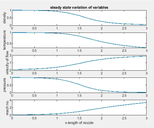
The graph received after reaching a steady state after 1400 time step, from both the form i.e conservative and non-conservative form are very similar to each other and very close to graph received by analyitcal solution.
2. Time-wise variation of the primitive variables
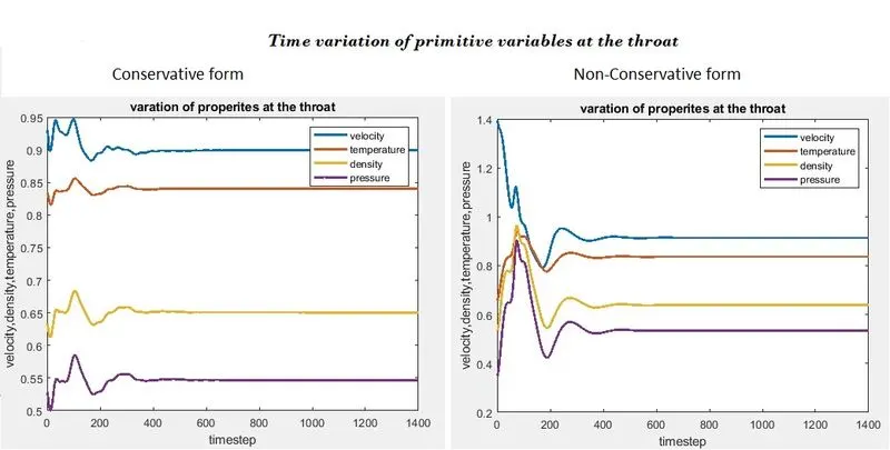
- Here we can see that , Initial time derivative are large , and oscillate in value. These oscillations are associated with various unsteady compression adn expansion waves which propagate through nozzle during transient process.
- At latter state after 800 time step time derivative got smaller and we have got the steady state resuts approximatley after 700 to 800 time step and their is negligeble variation after 1400 time step.
- We can here see that nonconservative form results are distinctly closer to the exact values as compare to nonconservative form resuts.
- And one more good thing with nonconservative form is that it converges to the result faster than conservative form .
3. Variation of Mass flow rate distribution inside the nozzle at different time steps during the time-marching process
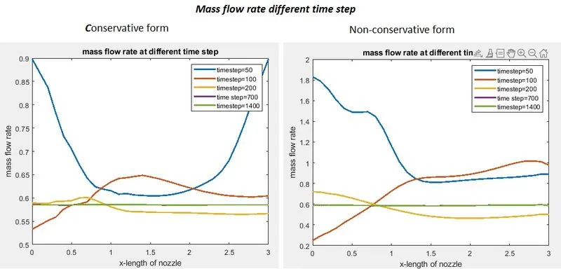
In both curves ; we can see that at and before 50th time step cure is looking distored and their is variation and after 50 the time step the mass flow distribution has chnged drastically.
At the 100th time step masss flow is still floping around inside the nozzle due to the transient variation of the flow field variables.
after 200 timestep the mass flow distribution is beginning to settle down and after 700 time steps the distribution is straight , horizonatla line across the graph at 1400 tim steps.
This says that the mass flow has converged to a constant , steady state value throughout the nozzle.
4. Comparison of Normalized mass flow rate distributions of both forms
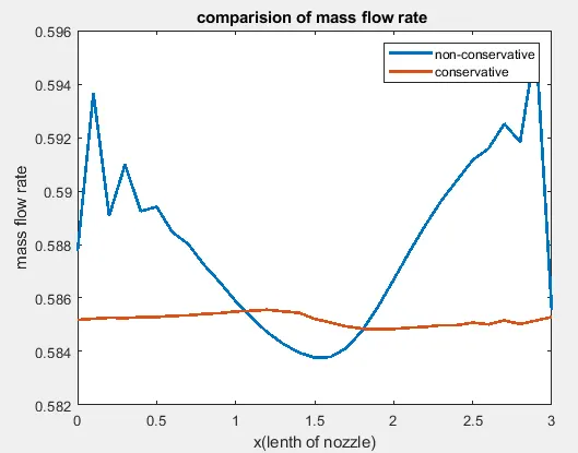 exact analytical solution for mass flow rate is = 0.579
Here the scale of the ordinate for mass flow rate is greatly magnified.
We can se that , conservative form gives result much closer to being a constant. In contrast, the nonconservative results have significant variations , specialy at the inflwo and outflow boundaries.
And the results form conservative form are , much closer to the exact analytical solutin of mass flow rate=0.579.
We can see that the steady state mass flow distribution by the conservative form is more satisfactory and nearest than that obtianed from the nonconservative form.
CONCLUSION:-
1.The conservative form does a better job in preserving mass throught the field, mainly because the mass flow itself is one of the dependent variables in the equations and mass flwo is a primary result frm these equations.
2.And nonconservative form does good in case with the primitive variables, because primiitve variables are dependent variables in it and mass flow is obtianed only as a secondary result.
Grid independene:Grid-independent means calculational results change so little along with a denser or looser grid that the truncation error can be ignored in numerical simulation.
3.From the table we can see that, for conservative form by doubling th number of grid pints the steady state numerical results are slightly closer to the exact analytical value(but still not as close as tthe nonconservation form results with half as may grid points).
4.The convergence rate is hihger in the conservative form as compae to nonconservative form.
5.This is because , in non conservaitve step in coding is less as compare to conservative form in which extra terms add which are later converted to desired result.