Week 3.5 - Deriving 4th order approximation of a 2nd order derivative using Taylor Table method

AIM:- To derive a fourth-order approximation for second-order derivative by

1. Central difference
2. Skewed right-side difference
3. Skewed left-side difference

Function f(x)=`e^x*cos(x)`

x=`pi/3`

`dx=(pi/4000,pi/40,20)`

Analytical second order derivative , f''(x)=`-2*e*sin(x)` ---------------------------------------1

GIVEN

i) The order of accuracy P = Number of nodes in the stencil N - order of derivative Q + 1 for symmetric/central schemes

ii) The order of accuracy P = Number of nodes in the stencil N - order of derivative Q for one-sided/skewed schemes

1.FOR THE CENTRAL SCHEME,

Number of nodes N= The order of accuracy P, + order of derivative Q -1

N = 4+2 -1 =5

`(dx)^2*(d^2u/dx^2)`=a*f(i-2) + b*f(i-1) + c*f(i) + d*f(i+1) + e*f(i+2)------------------------------------2

TYLOR TABLE

`(terms of Tylor series) / (function to evaluate)`	f(i)	dxf'(x)	(dx^2)f''(x)	(dx^3)f'''(x)	(dx^4)f''''(x)
af(i-2)	a	-2a	4a/2	-8a/6	16a/24
bf(i-1)	b	-b	b/2	-b/6	b/24
cf(i)	c	0	0	0	0
df(i+1)	d	d	d/2	d/6	d/24
ef(i+2)	e	2e	4e/2	8e/6	16e/24
SUM	0	0	1	0	0

solving above in MATLAB FOR a,b,c,d,& e

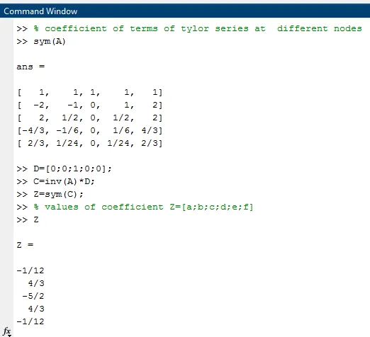
a=-1/12

b=4/3

c=-5/3

d=4/3

e=-1/12

`(dx)^2*(d^2u/dx^2)`=(-1/12)*f(i-2) + (4/3)*f(i-1) + (-5/3)*f(i) + (4/3)*f(i+1) + (-1/12)*f(i+2)------------------------------------3

2. FOR THE SKEWED RIGHT-SIDED SCHEME

Number of nodes N= The order of accuracy P, + order of derivative Q

N=4+2=6

`(dx)^2*(d^2u/dx^2) = a*f(i) + b*f(i+1) + c*f(i+2) + d*f(i+3) + e*f(i+4) + f*f(i+5)`---------------------------4

TYLOR TABLE

	f(i)	dxf'(x)	(dx^2)f''(x)	(dx^3)f'''(x)	(dx^4)f''''(x)	(dx^5)f'''''(x)	(dx^6)f'''''(x)
af(i)	a	0	0	0	0	0	0
bf(i+1)	b	b	b/2	b/6	b/24	b/120	b/720
cf(i+2)	c	2c	4c/2	8c/6	16c/24	32c/120	64c/720
df(i+3)	d	3d	9d/2	27d/6	81d/24	243d/120	729d/720
ef(i+4)	e	4e	16e/2	64e/6	256e/24	1024e/120	4096e/720
ff(i+5)	f	5f	25f/2	125f/6	625f/24	3125f/120	15625f/720
SUM	0	0	1	0	0	0	----

solving above in MATLAB FOR a,b,c,d,e,f

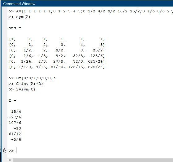
a=-15/4

b=-77/6

c=107/6

d=-13

e=61/12

f=-5/6

`(dx)^2*(d^2u/dx^2) = (-15/4)*f(i) + (-77/6)*f(i+1) + (107/6)*f(i+2) + (-13)*f(i+3) + (61/12)*f(i+4) + (-5/6)*f(i+5)`---------------------------5

3. For THE SKEWED LEFT-SIDED SCHEME

Number of nodes N= The order of accuracy P, + order of derivative Q

N=4+2=6

`(dx^2)*(d^2u/dx^2) = a*f(i-5) + b*f(i-4) + c*f(i-3) + d*f(i-2) + e*f(i-1) + f*f(i)`---------------------------------6

TYLOR TABLE

	f(i)	dxf'(x)	(dx^2)f''(x)	(dx^3)f'''(x)	(dx^4)f''''(x)	(dx^5)f'''''(x)	(dx^6)f'''''(x)
af(i-5)	a	-5a	25a/2	-125a/6	625a/24	-3125a/120	15625f/720
bf(i-4)	b	-4b	16b/2	-64b/6	256b/24	-1024b/120	4096e/720
cf(i-3)	c	-3c	9c/2	-27c/6	81c/24	-243c/120	729d/720
df(i-2)	d	-2d	4d/2	-8d/6	16d/24	-32d/120	64c/720
ef(i-1)	e	-e	e/2	-e/6	e/24	-e/120	b/720
ff(i)	f	0	0	0	0	0	0
SUM	0	0	1	0	0	0	-------

solving above in MATLAB FOR a,b,c,d,e,f

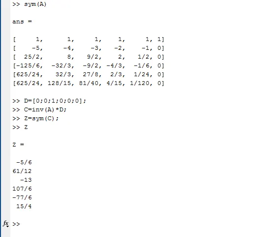
a=-5/6

b=61/12

c=-13

d=107/6

e=-77/6

f=15/4

`(dx^2)*(d^2u/dx^2) = (-5/6)*f(i-5) + (61/12)*f(i-4) + (-13)*f(i-3) + (107/6)*f(i-2) + (-77/6)*f(i-1) + (15/4)*f(i)`---------------------------------7

coding

now we will be evaluating second order derivatives with the help of the different scheme

clear all
close all
clc
%function f(x) = exp(x)*cos(x);
%analytical second order derivatives of f(x),f"(x)=-2exp(x)sin(x); at x=pi/3
x=pi/3;
dx=linspace(pi/4000,pi/40,20);

for i=1:length(dx)
   
    analytical_solution=-2*exp(x)*sin(x); % analytical solution of second order derivative 
    
    % central difference scheme
    
    %`(dx)^2*(d^2u/dx^2)`=(-1/12)*f(i-2) + (4/3)*f(i-1) + (-5/3)*f(i) + (4/3)*f(i+1) + (-1/12)*f(i+2)
    
    central_approx(i) =((-1/12)*(exp(x-2*dx(i))*cos(x-2*dx(i)))+(4/3)*(exp(x-dx(i))*cos(x-dx(i)))-(5/2)*(exp(x)*cos(x))+(4/3)*(exp(x+dx(i))*cos(x+dx(i)))-(1/12)*(exp(x+2*dx(i))*cos(x+2*dx(i))))/(dx(i))^2;
    
    error_central(i)=abs(central_approx(i) - analytical_solution); % comparing the outcome from central scheme to analytical scheme .
    
    % skewed right-side difference scheme
    
    % `(dx)^2*(d^2u/dx^2) = (-15/4)*f(i) + (-77/6)*f(i+1) + (107/6)*f(i+2) + (-13)*f(i+3) + (61/12)*f(i+4) + (-5/6)*f(i+5)`
    
   skewed_right(i)=((15/4)*(exp(x)*cos(x))-(77/6)*(exp(x+dx(i))*cos(x+dx(i)))+(107/6)*(exp(x+2*dx(i))*cos(x+2*dx(i)))-13*(exp(x+3*dx(i))*cos(x+3*dx(i)))+(61/12)*(exp(x+4*dx(i))*cos(x+4*dx(i)))-(5/6)*(exp(x+5*dx(i))*cos(x+5*dx(i))))/(dx(i))^2;
    
   error_skewed_right(i)=abs(skewed_right(i)-analytical_solution); % comparing the outcome with analytical solution and storing the error
   
   % skewed left side difference scheme
   %(dx^2)*(d^2u/dx^2) = (-5/6)*f(i-5) + (61/12)*f(i-4) + (-13)*f(i-3) + (107/6)*f(i-2) + (-77/6)*f(i-1) + (15/4)*f(i)`
   
   skewed_left(i)=((-5/6)*(exp(x-5*dx(i))*cos(x-5*dx(i)))+(61/12)*(exp(x-4*dx(i))*cos(x-4*dx(i)))-13*(exp(x-3*dx(i))*cos(x-3*dx(i)))+(107/6)*(exp(x-2*dx(i))*cos(x-2*dx(i)))-(77/6)*(exp(x-dx(i))*cos(x-dx(i)))+(15/4)*(exp(x)*cos(x)))/(dx(i))^2;
   
   error_skewed_left(i)=abs(skewed_left(i)-analytical_solution); % comparing the outcome with analytical solution and storing the error
   
end 
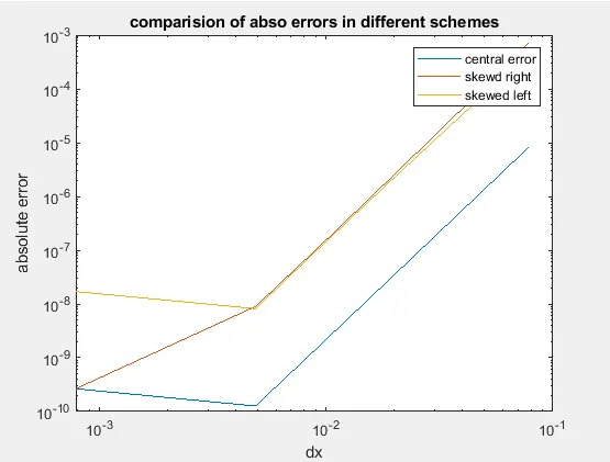
% we are  ploting the graph between the different vaues of dx and absolute
% errror occured in different schemes for each value of dx.

loglog(dx,error_central,dx,error_skewed_right,dx,error_skewed_left);
title('comparision of abso errors in different schemes')
xlabel('dx')
ylabel('absolute error')

legend('central error','skewd right','skewed left')

outcome

conclusion

1. from the graph it can be observed that the central difference has the least error as compared to other schemes.

2. the skewed right side scheme has the maximum error.

3. the skewed left side scheme error lies close to the skewed right but below it, i.e it has less error than skewed right.

error

skewed right side>skewed left side >central difference

Skewed difference scheme is more useful than central difference shceme because central difference can't be used at the boundary of the domain as it takes the value from both sides which is not possible at the boundary. but skewed take value from one side there for a combination of right and left-skewed and be used at boundary.

The skewed scheme is prefered over forward difference and backwards difference approximation because it is a higher-order approximation so the error is minimum.