Week 5.1 - Mid term project - Solving the steady and unsteady 2D heat conduction problem
AIM:- Steady-state and Transient state analysis of 2D heat conduction equation.
We will be using point iterative methods and will also use an explicit approach for transient equations.
Iterative methods to be used are :
- Jacobi
- Gauss-Seidel
- Successive over-relaxation(SOR)
Given :
`dT/dt + alpha*(d^2T/dx^2 +d^2T/dy^2) =0`--------Transient equation or Unsteady state equation of 2D heat conduction
`d^2T/dx^2 + d^2T/dx^2 =0`----------------Steady state equaiton of 2D heat conduction
Coefficeint of thermal conductivity (`alpha`) = 1.4 Watt/meter-kelvin ;
Absolute error used = 1e-4;
Area of domain =1 m^2` ;
Lenght of domain in X direction =1 m ;
Lenght of domain in Y direction =1 m ;
i = X direction
j = Y direction
nx = ny , are number nodes in x and y direction respectively (10-10) ;
dx = grid size in x direction = `L/(nx-1)`
dy = grid size in y direction = `L/(ny-1)`
Boundary condition :
Top Boundary = 600 K
Bottom Boundary = 900 K
Left Boundary = 400 K
Right Boundary = 800 K
At the corners of the domain, the temperature is taken as the average of the temperature of adjacent edges.
Calculation :
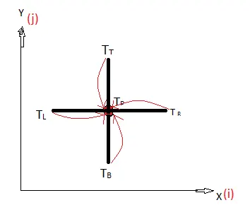 |
Notations used
`T(i-1,j)=TundersetL` and `T(i+1,j)=TundersetR`
`T(i,j-1)=TundersetB` and `T(i,j+1)=TundersetT`
`T(i,j)=TundersetP`
`d^2T/dx^2 + d^2T/dx^2 =0`---------------------Steady state eauaiton (2D)
Numerically discretizing the above equation
we will get,
`(T(i+1,j)-2*T(i,j)+T(i-1,j))/(Deltax)^2 + (T(i,j+1)-2*T(i,j)+T(i,j-1))/(Deltay)^2 =0`
T(i,j)=`(2*((Deltax^2 + Deltay^2)/(Deltax^2*Deltay^2)))^-1*((TundersetL``+ TundersetR`)`*1/(Deltax^2)`+ (`TundersetT` + T`TundersetB`)`*1/(Deltay^2)`) ; ----------1
K =`(2*((Deltax^2 + Deltay^2)/(Deltax^2*Deltay^2)))^-1`;
`dT/dt + alpha*(d^2T/dx^2 +d^2T/dy^2) =0`--------Transient equation or Unsteady state equation(2D)
Above equation can numerically disretize in two ways
1. Explicit 2. implicit
Here overset n means equation is being evaluated for `n overset (th)` time step and similarly of `(n+1)overset(th)` time step
k1`=(alpha*Deltat)/(Deltax)`
k2 =`(alpha*Deltat)/(Deltay)`
Explicit approach: The above-mentioned equation is evaluated by considering the values from the previous time step.
In explicit approach, only one variable is unknown that two is of next time step and rest variable are unknown from previous time step. Therefore this can be easily be solved.
`TundersetPoverset(n+1)` =`(1-2*k1-2*k2)*T(i,j)oversetn`+k1(`TundersetLoversetn`+`TundersetRoversetn`) + k2*(`TundersetToversetn`+`TundersetBoversetn`)
Implicit approach: The transient equation is solved by extracting values from the next time step which is not yet evaluated, so in this approach, we get a number of unknown variables.
and a system of linear equations is formed, to solve them iterative methods are being used. In all iterative processes, we have to initially assume or guess the values of variables.
1. Jacobi method. : In this the equation does uses the updated value of variables to solve a pair of variables.
2. gauss seidel; In this method, to solve an equation we use the updated value of the variable available from the previous iteration.
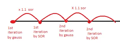
3. SOR: it is a modified form of Gauss seidel, and helps us to converge to our solution quickly. it Uses a variable which modiefied each iteration outcome.
`TundersetPoverset(n+1)` = (`TundersetPoversetn` + `k1*`(`TundersetLoverset(n+1)` + `Toverset(n+1)undersetR`) + k2*(`TundersetToverset(n+1)` + `TundersetBoverset(n+1)`)`*1/(1 +2*k1 + 2*k2)`
CODING
1. Steady-state
% solving the 2D steady-state heat conduction equation by using the point iterative method.
% d^2T/dx^2+d^2T/dx^2=0 , 2d steady-state equation
clear all
close all
clc

% defining no. of nodes in both the dimensions
nx=10; % in x direction
ny=10; % in y direction

%defining temperature in the domain of 1 square meter.
%Initial condition is being assumed i.e 300 k with the area.
T=300*ones(nx,ny);

% defining domain length with no. of grids in both direction i.e x=y= 1m
x=linspace(0,1,nx);
y=linspace(0,1,ny);

%Defining grid size
dx=x(2)-x(1);
dy=y(2)-y(1);


k=2*((dx)^2+(dy)^2)/(dx*dy)^2;

% defining boundary condition
T(1,:)=600;
T(end,:)=900;
T(:,1)=400;
T(:,end)=800;

% defining temperature at corners as the average of two adjacent edges of the boundaries.
T(1,1)=(400+600)/2;
T(1,end)=(600+800)/2;
T(end,end)=(900+800)/2;
T(end,1)=(900+400)/2;

% coping T
Told=T;  % help us to define the previous array of T

iterative_solve =3; % creating a variable to call it for different methods

% absolute error or tolerance in error exceptable
error=100;
tol=1e-4;

if (iterative_solve ==1) % this means this below function will be executed only when iterative_solve is equal to 1.
    jacobi_iter=1;
    %converging loop
    while (error > tol) % this while loop will execute itself until error coming is geater then tol defined.
        %space loop
        for i=2:nx-1
            for j=2:ny-1
                term1=(1/k)*(Told(i-1,j) + Told(i+1,j))/((dx)^2);
                term2=(1/k)*(Told(i,j-1) + Told(i,j+1))/((dy)^2);


                T(i,j)=(term1+term2);

            end
        end
        error=max(max(abs(Told - T))); % defining error for while loop
        %updating Told
        Told=T;
        jacobi_iter=jacobi_iter +1; % this will count no. of iteration took place to converge
    end
    contourf(x,y,T,'ShowText','on') % ploting a colured varient graph for T evaluted
    colormap(jet)
    title_text=sprintf('Jacobi iteration no.= %d',jacobi_iter); % trying to print no.of iteration took place as title of the graph.
    title(title_text)
    set(gca,'YDIR','reverse')
    colorbar
end


% for gauss siedal

if (iterative_solve ==2) % this means this below function will be executed only when iterative_solve is equal to 1.
    GS_iter=1
    %converging loop
    while (error > tol)
        %space loop
    for i=2:nx-1
     for j=2:ny-1
 % here we are taking repalacing Told(i-1,j) with T, beacuse Told(i-1,j) is being known  form previous iteration and being updated in T. and T(i+1,j) is still to be known so it is as it is.
         term1=(1/k)*(T(i-1,j) + Told(i+1,j))/((dx)^2);
similarly for T(i,j-1) to T(i,j-1)
        term2=(1/k)*(T(i,j-1) + Told(i,j+1))/((dy)^2);


        T(i,j)=(term1+term2);

     end
    end
    error=max(max(abs(Told - T)));
    %updating Told
        Told=T;
        GS_iter=GS_iter +1
    end
    contourf(x,y,T,'ShowText','on')
    colormap(jet)
    title_text=sprintf('gauss iteration no. = %d',GS_iter);
    title(title_text)

    set(gca,'YDIR','reverse')
    colorbar
end
% for SOR
w=1.1;%this help us to modify each and every value iteration to further extend and help us to converge fast

if (iterative_solve ==3)
    SOR_iter=1;
    %converging loop
    while (error > tol)
        %space loop
    for i=2:nx-1
     for j=2:ny-1
        term1=(1/k)*(T(i-1,j) + Told(i+1,j))/((dx)^2);
        term2=(1/k)*(T(i,j-1) + Told(i,j+1))/((dy)^2);
          G(i,j)=term1+term2;
   T(i,j)=(1-w)*Told(i,j)+w*G(i,j);
     end
    end
    error=max(max(abs(Told - T)));
    %updating Told
        Told=T;
        SOR_iter=SOR_iter +1;
    end
    contourf(x,y,T,'ShowText','on')
    colormap(jet)
    title_text=sprintf('SOR iteration no.= %d',SOR_iter);
    title(title_text)
    set(gca,'YDIR','reverse')
    colorbar
end
OUTPUT:
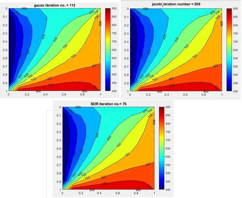
UNSTEADY STATE (IMPLICIT)
% Transient analysis of 2D heat conduction equatin by iterative process % solving the 2D steady heat onduction equation by using point iterative method.
% d^2T/dx^2+d^2T/dx^2=0
clear all
close all
clc
% definig no. of nodes in both the dimensions
nx=10;
ny=10;
%defining temperature in domain of 1 square meter.
T=300*ones(nx,ny);
x=linspace(0,1,nx);
y=linspace(0,1,ny);
%grid size
dx=x(2)-x(1);
dy=y(2)-y(1);
alpha=1.4;
dt=10; % dt can be anything thier , but reasonable
k1=(alpha*dt)/((dx)^2);
k2=(alpha*dt)/((dy)^2);
% defining boundary condition
T(1,:)=600;
T(end,:)=900;
T(:,1)=400;
T(:,end)=800;
% defining temperature at corners as average of two adjacent
T(1,1)=(400+600)/2;
T(1,end)=(600+800)/2;
T(end,end)=(900+800)/2;
T(end,1)=(900+400)/2;
% coping T
Told=T;
Tpre=T;
iterative_solve =3;
% absolute error or tolerance in error exceptable
error=2;
tol=1e-4;

if iterative_solve==1
    jacobi_iter=1;
   for t=1:1400
      error=2;

   %converging loop
    while (error > tol)
        %space loop
       for i=2:nx-1
        for j=2:ny-1

         term1=( 1+ (2*k1) + (2*k2) )^(-1);
         term2=k1*term1;
         term3=k2*term1;
         H=( Told(i-1,j) + Told(i+1,j) );
         V=( Told(i,j-1) + Told(i,j+1) );

         T(i,j)=((Tpre(i,j)*term1) + (H*term2) + (V*term3));

      end
     end
         error = max(max(abs(Told - T)));
         %updating Told
         Told=T;
         jacobi_iter = jacobi_iter +1;
   end
    Tpre = T;
    end
     contourf(x,y,T,'ShowText','on')
     colormap(jet)
     title_text=sprintf('jacobi_iteration number = %d',jacobi_iter);
     title(title_text)
     set(gca,'YDIR','reverse')
     colorbar
end


% f0r Gauss sideal

if iterative_solve==2
    GS_iter=1;
   for t=1:1400
      error=2;

   %converging loop
    while (error > tol)
        %space loop
       for i=2:nx-1
        for j=2:ny-1

         term1=( 1+ (2*k1) + (2*k2) )^(-1);
         term2=k1*term1;
         term3=k2*term1;
         H=( T(i-1,j) + Told(i+1,j) );
         V=( T(i,j-1) + Told(i,j+1) );

         T(i,j)=((Tpre(i,j)*term1) + (H*term2) + (V*term3));

      end
     end
         error = max(max(abs(Told - T)));
         %updating Told
         Told=T;
         GS_iter = GS_iter +1;


    end
    Tpre = T;
    end
     contourf(x,y,T,'ShowText','on')
     colormap(jet)
     title_text=sprintf('Gauss_iteration number = %d',GS_iter);
     title(title_text)
     set(gca,'YDIR','reverse')
     colorbar
end

% FOR SOR
w=1.4;

if iterative_solve==3
    SOR_iter=1;
   for t=1:1400

       error=2;

   %converging loop
    while (error > tol)
        %space loop
       for i=2:nx-1
        for j=2:ny-1

         term1=( 1+ (2*k1) + (2*k2) )^(-1);
         term2=k1*term1;
         term3=k2*term1;
         H=( T(i-1,j) + Told(i+1,j) );
         V=( T(i,j-1) + Told(i,j+1) );

        GS(i,j)=((Tpre(i,j)*term1) + (H*term2) + (V*term3));
        T(i,j)=(1-w)*(Told(i,j)) + w*(GS(i,j));

      end
     end
         error = max(max(abs(Told - T)));
         %updating Told
         Told=T;
         SOR_iter = SOR_iter +1;


    end
    Tpre = T;
    end
     contourf(x,y,T,'ShowText','on')
     colormap(jet)
     title_text=sprintf('SOR_iteration number = %d',SOR_iter);
     title(title_text)
     set(gca,'YDIR','reverse')
     colorbar
end 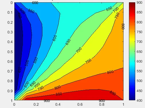
UNSTEADY STATE (EXPLICIT)
% Transient analysis of 2D heat conduction equation by time marching explicit
% dT/(dt)^2+(alpha)*(d^2T/dx^2+d^2T/dy^2)=0;
clear all
close all
clc
% definig no. of nodes in both the dimensions
nx=10;
ny=10;
%defining temperature in domain of 1 square meter.
T=300*ones(nx,ny);
x=linspace(0,1,nx);
y=linspace(0,1,ny);
%grid size
dx=x(2)-x(1);
dy=y(2)-y(1);
alpha=1.4;

% k1 + k2 <= 0.5 i.e cfl no. should be less than 0.5
dt=0.5/((alpha)/((dx)^2)+(alpha)/((dy)^2));

k1=(alpha*dt)/((dx)^2);
k2=(alpha*dt)/((dy)^2);

% defining boundary condition
T(1,:)=600;
T(end,:)=900;
T(:,1)=400;
T(:,end)=800;
% defining temperature at corners as average of two adjacent
T(1,1)=(400+600)/2;
T(1,end)=(600+800)/2;
T(end,end)=(900+800)/2;
T(end,1)=(900+400)/2;
% coping T
Told=T;

% time loop
for t=1:1400
    % space loop
    for i=2:nx-1
        for j=2:ny-1
            %  defining differnt terms used
            term1 = (1-(2*k1)-(2*k2))*Told(i,j);
            term2 = (k1)*(Told(i-1,j)+Told(i+1,j));
            term3 = (k2)*(Told(i,j-1)+Told(i,j+1));

            T(i,j)= term1 + term2 + term3;
        end
    end
    % udating value of T for text time step
   Told=T;

end
     contourf(x,y,T,'ShowText','on')
     colormap(jet)
     set(gca,'YDIR','reverse')
     colorbar
title('(EXPLICIT) FOR UNSTEADY STEADY') 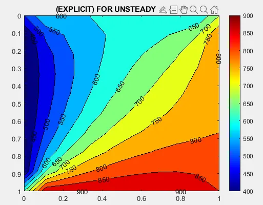
CONCLUSION
- AS we can see that all the outcomes form steady or unsteady equations and from all the iterative approaches are the same. The only difference is the number of iteration required to reach the solution.
- Irrespective of steady or unsteady analysis, the no. of iterations required by the Jacobi approach is the highest followed by Gauss seidel then SOR.
- JACOBI > GAUSS SIEDEL > SOR
| TYPE OF EQUATION | APPROACH | ITERATIVE METHOD | NO. OF ITERATIONS |
| STEADY-STATE | IMPLICIT |
Jacobi Gauss Siedel SOR |
208 112 76 |
| UNSTEADY STATE | IMPLICIT |
Jacobi Gauss Siedel SOR |
1749 1595 1483 |
- Jauss has a higher no. of iterations because it does intake the updated value of the variables in the equations to calculate the next variable which is being already evaluated, whereas Gauss seidel takes the values of all the variables which are already evaluated for the calculation of text variable. Therefore it Jacobi takes a large no. of iterations to converge then gauss.
- SOR is a modified form of Gauss, it just enhances the output from each iterative form gauss, which leads to quick convergence.
- NO ITERATION, STEADY STATE < UNSTEADY STATE
- One can notice that no. of iteration in steady-state is less than the unsteady state, this is because in steady-state there are only space terms (i.e x and y) whereas in unsteady-state there is the addition of rate of change of temperature term so the no. of variables in the unsteady state is more than steady-state therefore no. of iteration required to converge for the unsteady state is higher than steady-state.
- SO finally we can say that SOR gives result in less no. of iterations and steady state requires lesser no. of iteration .