Week 9 - FVM Literature Review

OBJECTIVE:- The project objective is to define the Finite Volume method and describe the difference between FVM and FDM. And also we describe the need for interpolation schemes and flux limiters in FVM.

DESCRIPTION OF THE PROJECT:- In CFD(Computational Fluid Mechanics), there are mainly three methods:-

• Finite Difference Method:- In numerical analysis, finite-difference methods are a class of numerical techniques for solving differential equations by approximating derivatives with finite differences. Both the spatial domain and time interval(if applicable) are discretized, or broken into a finite number of steps, and the value of the solutions at these discrete points is approximated by solving algebraic equations containing finite differences and values from nearby points.
• Finite Element Method:- The FEM is a general numerical method for solving partial differential equations in two or three space variables. To solve a problem, the FEM subdivides a large system into smaller, simpler parts that are called finite elements. This is achieved by a particular space discretization in the space dimensions, which is implemented by the construction of a mesh of the object, the numerical domain for the solution, which has a finite number of points. The FEM then approximates a solution by minimizing an associated error function via the calculus of variation.
• Finite Volume Method:- The finite volume method is a method for representing and evaluating partial differential equations in the form of algebraic equations. In the finite volume method, volume integrals in a partial differential equation that contain a divergence term are converted to surface integrals, using the divergence theorem. These terms are then evaluated as fluxes at the surfaces of each finite volume. Because the flux entering a given volume is identical to that leaving the adjacent volume, these methods are conservative. Finite volume refers to the small volume surrounding each node point on a mesh.

So now let’s discuss why FVM methods are more preferable than FDM or FEM for heat transfer and fluid mechanics community:-

A finite difference method (FDM) discretization is based upon the differential form of the PDE to be solved. Each derivative is replaced with an approximate difference formula that can generally be derived from a Taylor series expansion.

`f(x+∆x) = f(x) + (∆x) f’(x) + (∆x^2)/(2!) f’’(x) + (∆x^3)/(3!) f’’’(x) + …………………`

In this Taylor series expansion, we mainly rely on the smallness of `∆x`. So, if `∆x` is very very small, then we can get rid of the problem by truncating it up to a finite number of terms or up to very few terms. And if it is not so, then truncating the Taylor series up to a finite number of terms or up to very few terms can give rise to significant errors and that is one of the drawbacks of a Taylor series based discretization method, where the Taylor series itself truncated up to a few terms can give discrepancies, then if we use that as a basis of discretization that is bound to give rise to some sort of discrepancies. So that is not only the problem, we have some other problems also that is

• Conservativeness:-If the physical problem involves the conservation of variables, the discretized equation should reflect physically the same conservation. That means if we have a collection of discrete equations all together summed up, they should represent the conservation of the physical variable or the entire control volume. That means if it is a problem, where the physical requirement is momentum conservation, then the discretized equation summed up together over the entire domain that the equation must do. Now it is not granted from the finite difference method, it is just a mathematically expand Taylor series, where we have never enforced any requirement of conservation. Therefore, it is not a necessity that the finite difference discretization will satisfy the requirement of conservation. And conservativeness is not inbuilt as a part of the discretization of the finite difference method.
• Boundness:- So, let’s assume a rod, which have a finite temperature difference in both end side of the rod. Let us say that the left end is in touch with ice at 0-degree centigrade and the right end is in touch with steam at 100-degree centigrade. And let us say there is no heat source and heat sink and let us say we are interested in the temperature distribution. So, when we say that we are interested in the temperature distribution, whatever we get in between, should be bounded by its bounded values. We cannot expect something less than 0 and greater than 100 in between the rod. So it is a bounded nature of the solution, which comes from the physical description of the problem, that discretization also should ensure this boundedness, that is once we have discretized, our solution should automatically come out, which would ensure this boundedness that also we never ensured discretization policy of the finite difference method.
• Transportiveness:- If there is a predominant direction of flow, then properties should be having a predominant transport direction based on the flow direction. For example, if the flow has a high Reynolds number and if we have some property say enthalpy being transported. So, enthalpy will be predominantly transported along the direction of the flow. Of course, it will have some tendency to get transported along the opposite direction because of diffusion. Because diffusion is equally acting in all directions, but as it is predominantly fluid flow that is governing the behavior for high Reynolds number, it is the inertia effect that is more dominant. So it will try to have the effect of the transport predominantly in the direction of flow, where the Reynolds number is large. So with FDM we can't handle that type of problems.

To handle the complex geometry with the FDM method is very TDS. The finite element method is mathematically very rigorous, it can easily handle the complex geometry, but it does not carry the sense of conservativeness explicitly through its interpolation for fluid flow and heat transfer problems.

So how does the finite volume method solve those problems:-

1. Instead of writing the equations in a point, we write it for a volume.
2. Then, we apply few mathematical techniques to help us solve these equations for any type of grid.
3. Also, the finite volume representation preserves the concept of conservation.

Steps in FV discretization

• Step-1:- Divide the domain into several finite-size sub-domains. Each sub-domains are represented by a finite no of grid points.
• Step-2:- Integrate the governing differential equation over each sub-domain.
• Step-3:- Consider a profile assumption for the dependent variable for evaluating the above integrals and express the result in terms of algebraic quantities at the grid points.

To understand the Fvm scheme let's take 1D linear heat conduction equation as an example

`d/dx [k (dT)/(dx)]+S=0`

Where k is the thermal conductivity and S is the source term. Boundary values of T at points A and B are prescribed. An example of this type of process, we consider that one-dimensional heat conduction in a rod.

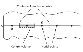
Step 1:- Grid generation

The first step in the finite volume method is to divide the domain into discrete control volumes. So, each control volume should be associated with a grid point. The centroid of each control volume we consider for the respective grid points and we also require boundaries of the control volumes because we also have to incorporate boundary conditions.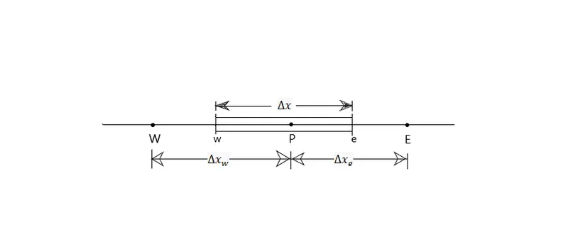

So, the main grid point of the control volume is given by P. On the left side, the neighbor point is W means West, and on the right side the neighbor point is E means East. And the face on the side of E is designated by lower case e and on the side of W, the face is designated by lower case w.

Step 2:- Integrate the gde

The next step is to integrate the governing differential equation over each control volume.

`∫_e^w{d/dx (k (dT)/dx)+S}dV=0`

`or,∫_e^wd/dx (k (dT)/dx).A dx+ ∫_e^wS dV=0` [here, dV = A.dx]

`or, [kA (dT)/dx]_e- [kA (dT)/dx]_w+ ∫_e^wS dV = 0`

Here A is the cross-sectional area of the control volume face and S is the the function of T. So, to get the corresponding algebraic equation, we must have profile variation for T as a function of x, so that we can calculate `(dT)/dx`. So, the problem boils down to some assumptions on how T varies with x. Since S is the function of a T so that we have to consider a profile of T for the source term and the finite volume method has a very attractive feature. We can use different profile assumptions for different terms because eventually, the profile assumption is required only for evaluating the necessary integrals. So now we go for the next step for profile assumptions and get the corresponding algebraic equation.

Step 3:- Profile assumption and solve the equation

Profile assumption or interpolation function is necessary to integrate the integral equation and once we integrate it, we will get the result as a function of T. We will start from the simplest profile assumption rather than a higher-order approximation of T as a function of x for calculating `(dT)/dx` .

Profile 1:-

So first profile assumption is a piecewise constant profile of T. So, we have a control volume. We have to remember that these values could have been useful, only in terms of the values at the respective grid points. Otherwise, it is artificial only at the respective grid points.

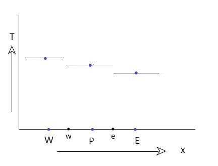
But this profile can’t work because of not the reason for such apparent discontinuities, but because of the reason that we require the value of `(dT)/dx` for our calculation. So, if T is constant we can’t get `(dT)/dx` , it will be zero.

Profile 2:-

The second profile assumption is piecewise linear but not a constant linear. We need to calculate `(dT)/dx` at e and w and in those points, `(dT)/dx` is discontinuous. So, we get two different derivatives for two different lines. It means k`(dT)/dx` is not continuous, it physically means that heat flux is not continuous. At a phase heat flux must be continuous means whatever heat flux enters the phase, the same heat flux should leave the phase but this discretization does not ensure that. So that is not an acceptable profile assumption.

Profile 3:-

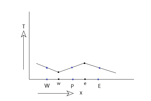
Instead of using a piecewise linear profile between the control volume phases, we consider the piecewise linear profile between the grid points.

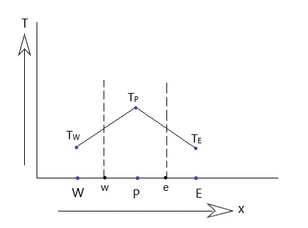
This will work because though in the point T_P, discontinuity is there but we don’t have to calculate `(dT)/dx` here. Our `(dT)/dx` the calculation is at these locations at the phases of the control volume, where the function is having continuous `(dT)/dx`. So this is a valid profile assumption.So we choose the Piecewise linear T between grid points profile to calculate `(dT)/dx`.

Now we go for choosing the profile assumption for S. S is a function of T and we choose the simplest profile for evaluating the S. So, we consider piecewise constant temperature within each control volume. Then we can approximate this T within the control volume as T at P. And thus we can consider the S within the control volume as S at P. And we consider `barS` is the average value of source S over the control volume.

Now we can go for converting the integral equation as an algebraic equation-

`[KA (dT)/dx]_e- [KA (dT)/dx]_w+∫_e^wS dV=0`

`or, K_e A (T_E-T_P)/(δx_e ) - K_w A(T_P- T_W)/(δx_e ) + barS ∆V = 0` [here, `barS ∆V` = `S_u + S_P T_P`]

`or, (K_e/(δx_e )+ K_w/(δx_w ))T_P = K_e/(δx_e ) T_E+ K_w/(δx_w ) T_W+ barS∆V`

We can write this equation like

a_PT_P = a_ET_E + a_WT_W + b ................(i)

`Where, a_E = (K_eA)/(δx_e ) , a_W = (K_wA)/(δx_w ) , b = barS∆V and a_P = a_E + a_W`

Discretised equations of the form must be set up at each of the nodal points to solve a problem. For control volumes that are adjacent to the domain boundaries the general discretized equation is modified to incorporate boundary conditions. The resulting system of linear algebraic equations is then solved to obtain the distribution of the property T at nodal points. Any suitable matrix solution technique may be enlisted for this task.

The need for interpolation schemes and flux limiters:-

Interpolation Scheme

The central differencing approximation has been used to represent the diffusion terms that appear on the right-hand side of the equation (i), and it seems logical to try linear interpolation to compute the cell face values for the convective terms on the left-hand side of this equation. The central difference scheme has many limitations. The Taylor series truncation error of the central differencing scheme is second-order. The requirement for positive coefficients in the central differencing scheme as given by the formula implies that the scheme will be stable and accurate only if Peclet number, Pe = F/D < 2. It is important to note that the cell Peclet number, as defined by (`Pe = F/D = (ρu Γ)/(δx)`), is a combination of fluid properties (ρ and Γ), a flow property (u) and a property of the computational grid (δx). So for given values of ρ and Γ, it is only possible to satisfy condition (`F_e/D_e = Pe_e < 2`) if the velocity is small, hence in diffusion-dominated low Reynolds number flows, or if the grid spacing is small. Owing to this limitation central differencing is not a suitable discretization practice for general-purpose flow calculations. This creates the need for discretization schemes that possess more favorable properties.

Flux limiters

Schemes of third-order and above have been developed for the discretization of convective terms with varying degrees of success. Implementation of boundary conditions can be problematic with such higher-order schemes. The fact that the QUICK scheme and other higher-order schemes can give undershoots and overshoots has led to the development of second-order schemes that avoid these problems. The class of TVD (total variation diminishing) schemes have been specially formulated to achieve oscillation-free solutions and have proved to be useful in CFD calculations. To make the scheme TVD, we must constrain or limit the range of possible values of the additional convective flux, that’s why we use a limiter function that was originally introduced to make the scheme higher-order. Hence, this limiter function is called a flux limiter function.

The flux limiter function for a scheme dictates the order of the scheme and its boundedness properties. Any second-order limited scheme could be based on a limiter function. A limiter function that satisfies the symmetry property ensures that backward- and forward-facing gradients are treated in the same fashion without the need for special coding.