Week 11 - Simulation of Flow through a pipe in OpenFoam
AIM:- The project aims to simulate an axisymmetric flow by applying the wedge boundary condition.
OBJECTIVE:- The objective is to simulate an axisymmetric flow by applying the wedge boundary condition. The flow is laminar and flows through a constant cross-section pipe at an inlet Reynold's number of 2100. Here, we do a steady-state simulation and we will validate our results with the Hagen- Poiseuille's equations for the fully developed flow.
We simulate our laminar flow in OpenFOAM. And to do that we will make our blockMeshDict file in MATLAB. And we compare the results which we get from OpenFOAM with the numerical result.
PROJECT DESCRIPTION:-
At first, we have to understand some theory parts related to our project. So,
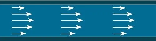
Laminar Flow:- Laminar flow is a flow where the streamlines are smooth and parallel to each other and flow is a highly ordered motion. At low velocities, the fluid tends to flow without lateral mixing, and adjacent layers slide past one another like playing cards. There are no cross-currents perpendicular to the direction of flow, nor eddies or swirls of fluids. In laminar flow, the motion of the particles of the fluid is very orderly with all particles moving in straight lines parallel to the pipe walls. We see this flow from the below figure(a)-
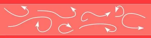
Turbulent Flow:- Turbulent flow is a flow where the streamlines are not smooth, the velocity fluctuations and highly disordered motion. It is a flow regime characterized by chaotic property changes. This includes a rapid variation of pressure and flows velocity in space and time. In contrast to laminar flow, the fluid no longer travels in layers, and mixing across the tube is highly efficient. We see this flow from the below figure(b)-
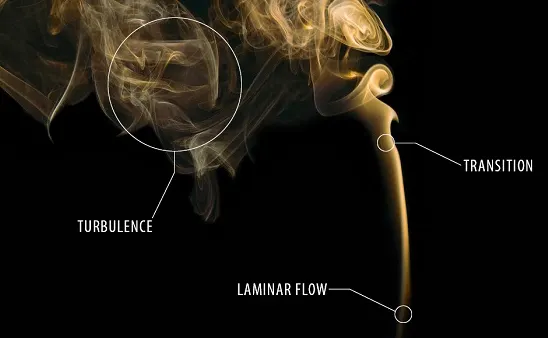
If we have been around smokers, we probably noticed that the cigarette smoke rises in a smooth plume for the first few centimeters and then starts fluctuating randomly in all directions as it continues its rise. So, that is one of the exammple of laminar and turbulent flow.
Reynolds number:- The Reynolds number represents the ratio of inertial forces to viscous forces and is a convenient parameter for predicting if a flow condition will be laminar or turbulent. It is defined as a characteristic length multiplied by a characteristic velocity and divided by the kinematic viscosity.
`Re_D` = `("Inertial Forces")/("Viscous Forces")`
= `(ρVD)/μ` = `(VD)/nu`
The Reynolds number at which the flow becomes turbulent is called the critical Reynolds number, `Re_(cr)`. The value of the critical Reynolds number is different for different geometries and flow conditions. For internal flow in a circular pipe, the generally accepted value of the critical Reynolds number is `Re_(cr) = 2300`. Under most practical conditions, the flow in a circular pipe is laminar for Re ≲ 2300, turbulent for Re ≳ 4000, and transitional in between. That is,
(Re ≲ 2300) - laminar flow
(2300 ≲ Re ≲ 4000) - transitional flow
(Re ≳ 4000) - turbulent flow
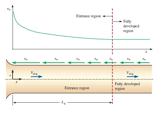
Fully Developed Flow:- Fully developed flow occurs when the viscous effects due to the shear stress between the fluid particles and pipe wall create a fully developed velocity profile. The region from the pipe inlet to the point at which the velocity profile is fully developed is called the hydrodynamic entrance region. Flow in the entrance region is called hydrodynamically fully developed flow since this is the region where the velocity profile develops.
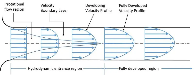
Entrance Length:- The entry length is the distance a flow travels after entering a pipe before the flow becomes fully developed. Entrance length refers to the length of the entry region, the area following the pipe entrance where effects originating from the interior wall of the pipe propagate into the flow as an expanding boundary layer. When the boundary layer expands to fill the entire pipe, the developing flow becomes a fully developed flow, where flow characteristics no longer change with increased distance along the pipe.
The hydrodynamic entry length is usually taken to be the distance from the pipe entrance to where the wall shear stress reaches within about 2 percent of the fully developed value. In laminar flow, the nondimensional hydrodynamic entry length is given approximately as,
`L_(h,"laminar")/D ≅0.05Re`
In turbulent flow, the intense mixing during random fluctuations usually overshadows the effects of molecular diffusion. The nondimensional hydrodynamic entry length for turbulent flow is approximated as,
`L_(h,"turbulent")/D=1.359(Re)^(1/4)`
Since our project is mainly based on the laminar flow, so we are now going to more discussion on the properties of laminar flow through a circular pipe.
Velocity profile for the laminar flow through a circular pipe:- The flow is fully developed if the pipe is sufficiently long (relative to the entry length) so that the entrance effects are negligible. In this section, we consider the steady, laminar, incompressible flow of fluid with constant properties in the fully developed region of a straight circular pipe. We obtain the momentum equation by applying a momentum balance to a differential volume element and we obtain the velocity profile by solving it.
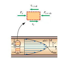
This is a free-body diagram of a ring-shaped differential fluid element of radius r, thickness dr, and length dx oriented coaxially with a horizontal pipe in fully developed laminar flow.
The velocity profile is fully developed laminar flow in a pipe is parabolic with a maximum at the centerline and a minimum (zero) at the pipe wall. After simplifying all the mathematical expressions we get the velocity profile expression which is,
`U(r) = - R^2/(4μ) ((dp)/dx)(1- r^2/R^2 )`
or, `U(r) = 2V_(avg)(1 - r^2/R^2 )` ..............(i)
This is a convenient form for the velocity profile since Vavg can be determined easily from the flow rate information. The maximum velocity occurs at the centerline and is determined from Eq.(i) by substituting r = 0,
`U_(max) = 2V_(avg)`
Therefore, the average velocity in fully developed laminar pipe flow is one-half of the maximum velocity.
Pressure Drop:- A quantity of interest in the analysis of pipe flow is the pressure drop P since it is directly related to the power requirements of the fan or pump to maintain flow. We note that `(dP)/dx` = constant, and integrating from `x = x_1` where the pressure is `P_1` to `x = x_1 + L` where the pressure is `P_2` gives
`∆P=P_2-P_1`
or, `(dP)/dx= (P_2-P_1)/L`
Hagen–Poiseuille’s Equation:- The Hagen–Poiseuille Equation is a fluidic law to calculate flow pressure drop in a long cylindrical pipe and it was derived separately by Poiseuille and Hagen in 1838 and 1839, respectively. The equation is
`∆P=P_2-P_1= (8μLV_(avg))/R^2`
`= (32μLV_(avg))/D^2`
Where `μ` is the fluid viscosity, L is the length of the pipe(> entry length), `V_(avg)` is the average velocity, R is the radius of the pipe and D is the diameter of the pipe. The Hagen–Poiseuille equation describes the relationship between pressure, fluidic resistance, and flow rate, analogous to voltage, resistance, and current, respectively, in Ohm’s law for electrical circuits (V=RI">V=RI).
Here, one thing we should notice is that fluid viscosity `mu` is proportional to the pressure drop. If `mu` is zero then `∆P` is also zero. Therefore, the drop of pressure from P1 to P2, in this case, is due entirely to viscous effects.
Assumptions:-
- Flow is Laminar
- The working fluid is incompressible and we choose here water as working fluid.
- The viscosity of water, mu = 0.00089 kg·m−1s−1
- The density of water, = 1000 kg/m^3
- The kinematic viscosity of water, `nu = mu/(rho)`
- Pipe diameter, D = 0.02
- The entry length, `L_h = 0.05*Re*D`
- The pipe length, L = Lh + 0.25
- Average velocity,`V_(avg) = (nu*Re)/D`
- Maximum velocity, `V_(max) = 2*V_(avg)`
- Pressure Drop,`∆P = (32μLV_(avg))/D^2`
- Kinematic Pressure, `P =(Delta P) /(rho)`
This assumption helps us to ready the geometry and choose the best solver for solving our equations. We choose icoFoam as a solver because it is a solver for laminar incompressible flow. In icoFoam solver we use cavity file for our project.
So, now we create our blockMeshDict file in MATLAB,
clear all;
close all;
clc;

Re = 2100;          % Reynolds number
Rho = 1000;         % Density of water
mu = 0.00089;       % Dynamic viscosity of water
nu = mu/Rho;        % Kinematic viscosity of water
D = 0.02;         % Diameter of the pipe
R = D/2;            % Radius of the pipe
ent_L = 0.05*Re*D;  % Entry length
theta = 4;          % Wedge angle in degree(It should be less than 5)

%Boundery condition
V_avg = (nu*Re)/D;             %Average velocity
V_max = 2*V_avg;               % Maximum velocity
L = ent_L + 0.25;              %Length of the pipe
Dell_P = (32*mu*L*V_avg)/D^2;  % Pressure drop
kin_P = Dell_P/Rho;            % Kinematic pressure drop

%Defining the points
v_0 = [0 0 0];
v_1 = [0 R*cosd(theta/2) R*sind(theta/2)];
v_2 = [0 R*cosd(theta/2) -R*sind(theta/2)];
v_3 = [L 0 0];
v_4 = [L R*cosd(theta/2) R*sind(theta/2)];
v_5 = [L R*cosd(theta/2) -R*sind(theta/2)];

%% creating a blockmeshh file
F_1 = '/*--------------------------------*- C++ -*----------------------------------*\';
F_2 = ' =========                 |';
F_3 = ' \\      /  F ield         | OpenFOAM: The Open Source CFD Toolbox';
F_4 = '  \\    /   O peration     | Website:  https://openfoam.org';
F_5 = '   \\  /    A nd           | Version:  9';
F_6 = '    \\/     M anipulation  |';
F_7 = '\*---------------------------------------------------------------------------*/';

F_8 = '// * * * * * * * * * * * * * * * * * * * * * * * * * * * * * * * * * * * * * //';

f1 = fopen('blockMeshDict.txt','w');

fprintf(f1,"%s\n",F_1);
fprintf(f1,"%s\n",F_2);
fprintf(f1,"%s\n",F_3);
fprintf(f1,"%s\n",F_4);
fprintf(f1,"%s\n",F_5);
fprintf(f1,"%s\n",F_6);
fprintf(f1,"%s\n",F_7);

fprintf(f1,"%s\n",'FoamFile');
fprintf(f1,"%s\n",'{');
fprintf(f1, "%11s %9s\n",'version','2.0;');
fprintf(f1, "%10s %12s\n",'format','ascii;');
fprintf(f1, "%9s %18s\n",'class','dictionary;');
fprintf(f1,"%10s %20s\n",'object','blockMeshDict;');
fprintf(f1,"%s\n",'}');
fprintf(f1,"%s\n\n",F_8);
fprintf(f1,"%s\n\n",'convertToMeters 1;');

fprintf(f1,"%s\n",'vertices');
fprintf(f1,"%s\n\n",'(');
fprintf(f1,"\t(%f %f %f)\n",v_0);
fprintf(f1,"\t(%f %f %f)\n",v_1);
fprintf(f1,"\t(%f %f %f)\n",v_2);
fprintf(f1,"\t(%f %f %f)\n",v_3);
fprintf(f1,"\t(%f %f %f)\n",v_4);
fprintf(f1,"\t(%f %f %f)\n\n",v_5);

fprintf(f1,"%s\n\n",');');

fprintf(f1,"%s\n",'blocks');
fprintf(f1,"%s\n",'(');
fprintf(f1,"\t%s %s\n",'hex (0 2 1 0 3 5 4 3) (50 1 200)', 'simpleGrading (0.2 1 1)');
fprintf(f1,"%s\n\n",');');

fprintf(f1,"%s\n",'edges');
fprintf(f1,"%s\n", '(');
fprintf(f1,"\t%s (%f %f %f)\n",'arc 1 2',0,R,0);
fprintf(f1,"\t%s (%f %f %f)\n",'arc 4 5',L,R,0);
fprintf(f1, "%s\n\n",');');

fprintf(f1,"%s\n",'boundary');
fprintf(f1,"%s\n",'(');

fprintf(f1,"\t%s\n","inlet");
fprintf(f1,"\t%s\n",'{');
fprintf(f1,"\t\t%s\n",'type patch;');
fprintf(f1,"\t\t%s\n",'faces');
fprintf(f1,"\t\t%s\n",'(');
fprintf(f1,"\t\t\t(%d %d %d %d)\n",0,1,2,0);
fprintf(f1,"\t\t%s\n",');');
fprintf(f1,"\t%s\n",'}');

fprintf(f1,"\t%s\n","outlet");
fprintf(f1,"\t%s\n",'{');
fprintf(f1,"\t\t%s\n",'type patch;');
fprintf(f1,"\t\t%s\n",'faces');
fprintf(f1,"\t\t%s\n",'(');
fprintf(f1,"\t\t\t(%d %d %d %d)\n",3,4,5,3);
fprintf(f1,"\t\t%s\n",');');
fprintf(f1,"\t%s\n",'}');

fprintf(f1,"\t%s\n","front");
fprintf(f1,"\t%s\n",'{');
fprintf(f1,"\t\t%s\n",'type wedge;');
fprintf(f1,"\t\t%s\n",'faces');
fprintf(f1,"\t\t%s\n",'(');
fprintf(f1,"\t\t\t(%d %d %d %d)\n",0,3,4,1);
fprintf(f1,"\t\t%s\n",');');
fprintf(f1,"\t%s\n",'}');

fprintf(f1,"\t%s\n","back");
fprintf(f1,"\t%s\n",'{');
fprintf(f1,"\t\t%s\n",'type wedge;');
fprintf(f1,"\t\t%s\n",'faces');
fprintf(f1,"\t\t%s\n",'(');
fprintf(f1,"\t\t\t(%d %d %d %d)\n",0,2,5,3);
fprintf(f1,"\t\t%s\n",');');
fprintf(f1,"\t%s\n",'}');

fprintf(f1,"\t%s\n","pipe");
fprintf(f1,"\t%s\n",'{');
fprintf(f1,"\t\t%s\n",'type wall;');
fprintf(f1,"\t\t%s\n",'faces');
fprintf(f1,"\t\t%s\n",'(');
fprintf(f1,"\t\t\t(%d %d %d %d)\n",1,4,5,2);
fprintf(f1,"\t\t%s\n",');');
fprintf(f1,"\t%s\n",'}');

fprintf(f1,"\t%s\n","axis");
fprintf(f1,"\t%s\n",'{');
fprintf(f1,"\t\t%s\n",'type empty;');
fprintf(f1,"\t\t%s\n",'faces');
fprintf(f1,"\t\t%s\n",'(');
fprintf(f1,"\t\t\t(%d %d %d %d)\n",3,0,0,3);
fprintf(f1,"\t\t%s\n",');');
fprintf(f1,"\t%s\n",'}');

fprintf(f1,"%s\n",');');

fprintf(f1,"%s\n",'mergePatchPairs');
fprintf(f1,"%s\n",'(');
fprintf(f1,"%s\n\n",');');
fprintf(f1,"%s",F_8);
blockMeshDict File
/*--------------------------------*- C++ -*----------------------------------*\
 =========                 |
 \\      /  F ield         | OpenFOAM: The Open Source CFD Toolbox
  \\    /   O peration     | Website:  https://openfoam.org
   \\  /    A nd           | Version:  9
    \\/     M anipulation  |
\*---------------------------------------------------------------------------*/
FoamFile
{
    version      2.0;
    format       ascii;
    class        dictionary;
    object       blockMeshDict;
}
// * * * * * * * * * * * * * * * * * * * * * * * * * * * * * * * * * * * * * //

convertToMeters 1;

vertices
(

	(0.000000 0.000000 0.000000)
	(0.000000 0.009994 0.000349)
	(0.000000 0.009994 -0.000349)
	(2.350000 0.000000 0.000000)
	(2.350000 0.009994 0.000349)
	(2.350000 0.009994 -0.000349)

);

blocks
(
	hex (0 2 1 0 3 5 4 3) (50 1 200) simpleGrading (0.2 1 1)
);

edges
(
	arc 1 2 (0.000000 0.010000 0.000000)
	arc 4 5 (2.350000 0.010000 0.000000)
);

boundary
(
	inlet
	{
		type patch;
		faces
		(
			(0 1 2 0)
		);
	}
	outlet
	{
		type patch;
		faces
		(
			(3 4 5 3)
		);
	}
	front
	{
		type wedge;
		faces
		(
			(0 3 4 1)
		);
	}
	back
	{
		type wedge;
		faces
		(
			(0 2 5 3)
		);
	}
	pipe
	{
		type wall;
		faces
		(
			(1 4 5 2)
		);
	}
	axis
	{
		type empty;
		faces
		(
			(3 0 0 3)
		);
	}
);
mergePatchPairs
(
);

// * * * * * * * * * * * * * * * * * * * * * * * * * * * * * * * * * * * * * //
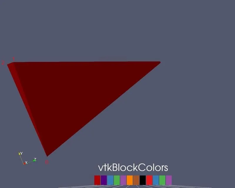
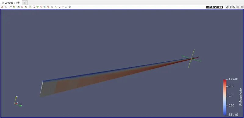
After creating blockMeshDict file the geometry looks like :-
Velocity File
/*--------------------------------*- C++ -*----------------------------------*\
  =========                 |
  \\      /  F ield         | OpenFOAM: The Open Source CFD Toolbox
   \\    /   O peration     | Website:  https://openfoam.org
    \\  /    A nd           | Version:  9
     \\/     M anipulation  |
\*---------------------------------------------------------------------------*/
FoamFile
{
    format      ascii;
    class       volVectorField;
    object      U;
}
// * * * * * * * * * * * * * * * * * * * * * * * * * * * * * * * * * * * * * //

dimensions      [0 1 -1 0 0 0 0];

internalField   uniform (0 0 0);

boundaryField
{
    inlet
    {
        type            fixedValue;
        value           uniform (0.0934 0 0);
    }

    outlet
    {
        type            zeroGradient;
    }

    front
    {
        type            wedge;
    }
    back
    {
        type            wedge;
    }
    pipe
    {
        type            noSlip;
    }
    axis
    {
        type            empty;
    }
}

// ************************************************************************* //
Pressure File - Here we use Kinematic pressure where,
Kinematic Pressure = `"Pressure Drop"/"Density"`= `(Delta P)/rho`
/*--------------------------------*- C++ -*----------------------------------*\
  =========                 |
  \\      /  F ield         | OpenFOAM: The Open Source CFD Toolbox
   \\    /   O peration     | Website:  https://openfoam.org
    \\  /    A nd           | Version:  9
     \\/     M anipulation  |
\*---------------------------------------------------------------------------*/
FoamFile
{
    format      ascii;
    class       volScalarField;
    object      p;
}
// * * * * * * * * * * * * * * * * * * * * * * * * * * * * * * * * * * * * * //

dimensions      [0 2 -2 0 0 0 0];

internalField   uniform 0;

boundaryField
{
    inlet
    {
        type            zeroGradient;
    }

    outlet
    {
        type            fixedValue;
        value           uniform 0.0156;
    }

    front
    {
        type            wedge;
    }
    back
    {
        type            wedge;
    }
    pipe
    {
        type            zeroGradient;
    }

    axis
    {
        type            empty;
    }
}

// ************************************************************************* //
Kinematic Viscosity - This file carry the properties of fluid. Here our working fluid is water and the kinematic visosity is approximately 1.7e-6.
/*--------------------------------*- C++ -*----------------------------------*\
  =========                 |
  \\      /  F ield         | OpenFOAM: The Open Source CFD Toolbox
   \\    /   O peration     | Website:  https://openfoam.org
    \\  /    A nd           | Version:  9
     \\/     M anipulation  |
\*---------------------------------------------------------------------------*/
FoamFile
{
    format      ascii;
    class       dictionary;
    location    "constant";
    object      transportProperties;
}
// * * * * * * * * * * * * * * * * * * * * * * * * * * * * * * * * * * * * * //

nu              [0 2 -1 0 0 0 0] 1.7e-6;


// ************************************************************************* //
Controldict File
/*--------------------------------*- C++ -*----------------------------------*\
  =========                 |
  \\      /  F ield         | OpenFOAM: The Open Source CFD Toolbox
   \\    /   O peration     | Website:  https://openfoam.org
    \\  /    A nd           | Version:  9
     \\/     M anipulation  |
\*---------------------------------------------------------------------------*/
FoamFile
{
    format      ascii;
    class       dictionary;
    location    "system";
    object      controlDict;
}
// * * * * * * * * * * * * * * * * * * * * * * * * * * * * * * * * * * * * * //

application     icoFoam;

startFrom       startTime;

startTime       0;

stopAt          endTime;

endTime         10;

deltaT          0.001;

writeControl    timeStep;

writeInterval   20;

purgeWrite      0;

writeFormat     ascii;

writePrecision  6;

writeCompression off;

timeFormat      general;

timePrecision   6;

runTimeModifiable true;


// ************************************************************************* //
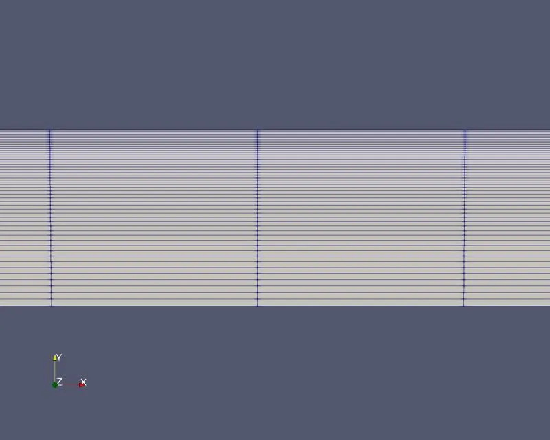
After running the file The mesh looks like:-
RESULTS:-
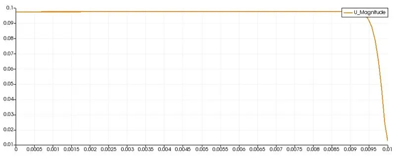
Velocity Profile at distance 1.175
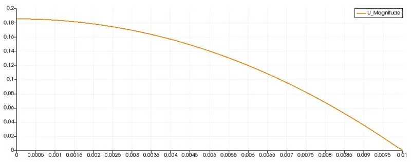
Velocity Profile at distance 2.3
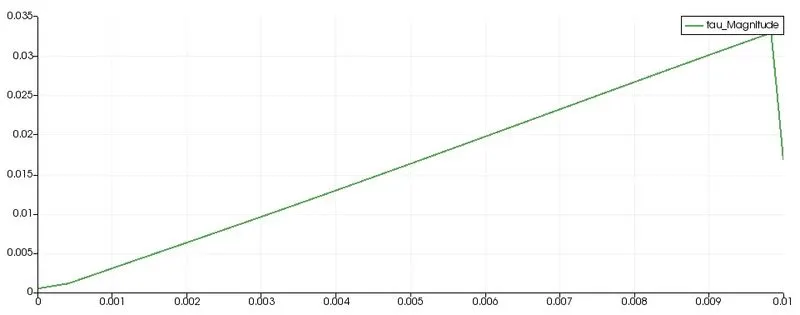
Shear stress plot at distance 2.3
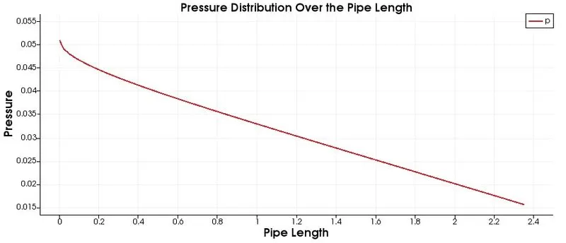
Pressure Distribution Over the Pipe Length
Now we check the validation of our results. For that we do numerical analysis in MATLAB
clear all;
close all;
clc;

Re = 2100;          % Reynolds number
Rho = 1000;         % Density of water
mu = 0.00089;       % Dynamic viscosity of water
nu = mu/Rho;        % Kinematic viscosity of water
D = 0.02;         % Diameter of the pipe
R = D/2;            % Radius of the pipe
ent_L = 0.05*Re*D;  % Entry length
theta = 4;          % Wedge angle in degree(It should be less than 5)

%Boundery condition
V_avg = (nu*Re)/D;             %Average velocity
V_max = 2*V_avg;               % Maximum velocity
L = ent_L + 0.25;              %Length of the pipe
Dell_P = (32*mu*L*V_avg)/D^2;  % Pressure drop
kin_P = Dell_P/Rho;            % Kinematic pressure drop

r = linspace(0,R,100);
for i = 1:length(r)
    U(i) = 2*V_avg*(1-(r(i)^2)/(R^2));
    tau(i) = 2*mu*V_max*(abs(r(i)))/R^2;

end
%shear stress
figure(1)
plot(r,tau,"r*","LineWidth",1)
xlabel("Radius","FontWeight","bold")
ylabel("Shear stress","FontWeight","bold")
title("Shear stress Analysis")

figure(2)
plot(r,U,"g*","LineWidth",1);
xlabel("Radius","FontWeight","bold")
ylabel("Velocity","FontWeight","bold")
title("Velocity Profile Validation Analysis")
Numerical results are
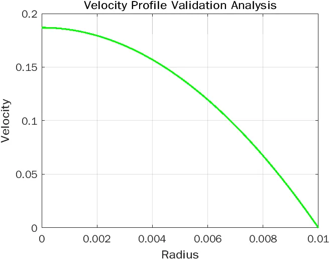
This is Velocity plot for fully developed flow:-
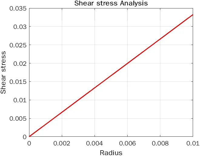
This is the Shear stress plot for fully developed flow:-
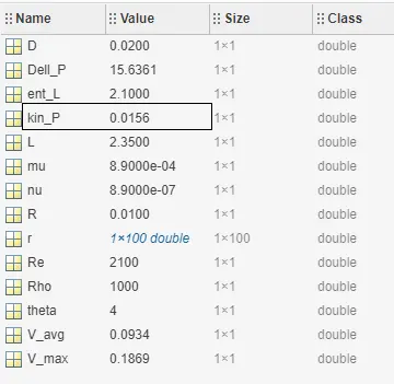
Kinematic Pressure value for our project
CONCLUSION:-
- If we compare the velocity profile, in the analytical result section we see two different velocity profiles at different pipe sections. It’s because the entry length is 2.1, so we see fully developed flow after 2.1 distance. In previous sections, the flow is developing. That’s why we see the different velocity profiles, one is before fully developed flow and another is after fully developed flow. And for fully developed flow the numerical and analytical velocity plot is the same.
- So, if we compare the analytical plot of shear stress and the numerical plot of shear stress are often the same plots but in the analytical shear stress plot after a certain radius, it’s falling. It’s because the calculation error of OpenFoam is just and nothing else.
- In the Analytical case, Pressure Drop in between 0.05 to 0.015. And we know in OpenFoam the pressure is Kinematic Pressure. In the Numerical result, the Kinematic pressure is 0.0156 and this is in between 0.05 to 0.015.