Week 5.1 - Mid term project - Solving the steady and unsteady 2D heat conduction problem
2D HEAT CONDUCTION EQUATION SOLUTION :-
2D heat conduction equation is classified as 2 types - A) Steady State Equation
B) Transient State Equation
Those equations we solve using Finite Difference Method. And here we apply a boundery condition on the equation which is
Top Boundary = 600 K
Bottom Boundary = 900 K
Left Boundary = 400 K
Right Boundary = 800 K
A) Steady State Equatioon :-
2D heat conduction steady-state equation is
`(d^2T)/(dx^2) + (d^2T)/(dy^2) = 0`
So, `T(i,j) = (1/k)((T(i-1,j) + T(i+1,j))/(dx^2)) + (1/k)((T(i ,j-1) + T(i,j+1))/(dy^2))`
where k = `2((dx^2 + dy^2)/(dx^2.dy^2))`
We solve the steady-state equation using an iterative method and mainly we use three types of an iterative method
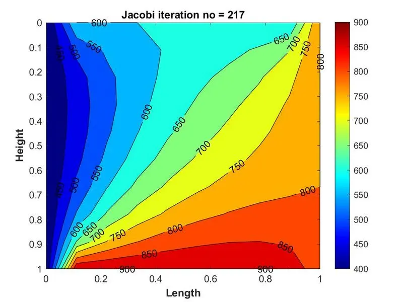
i) Jacobi Iterative method:- In numerical linear algebra, the Jacobi method is an iterative algorithm for determining the solutions of a strictly diagonally dominant system of linear equations. Each diagonal element is solved for, and an approximate value is plugged in. The process is then iterated until it converges.
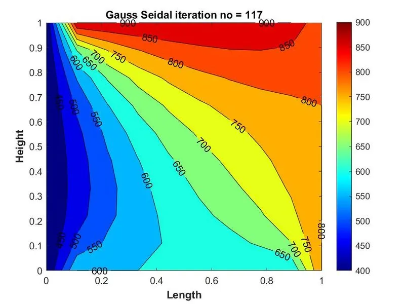
ii) Gauss-Seidel Iterative Method:- In numerical linear algebra, the Gauss-Seidel method, also known as the Liebmann methodor the method of successive displacement, is an iterative method used to solve a system of linear equations. It is named after the German mathematician's Carl Friedrich Gauss and Philipp Ludwig von Seidel, and it has a very small difference from the Jacobi method it is also comparatively fast.
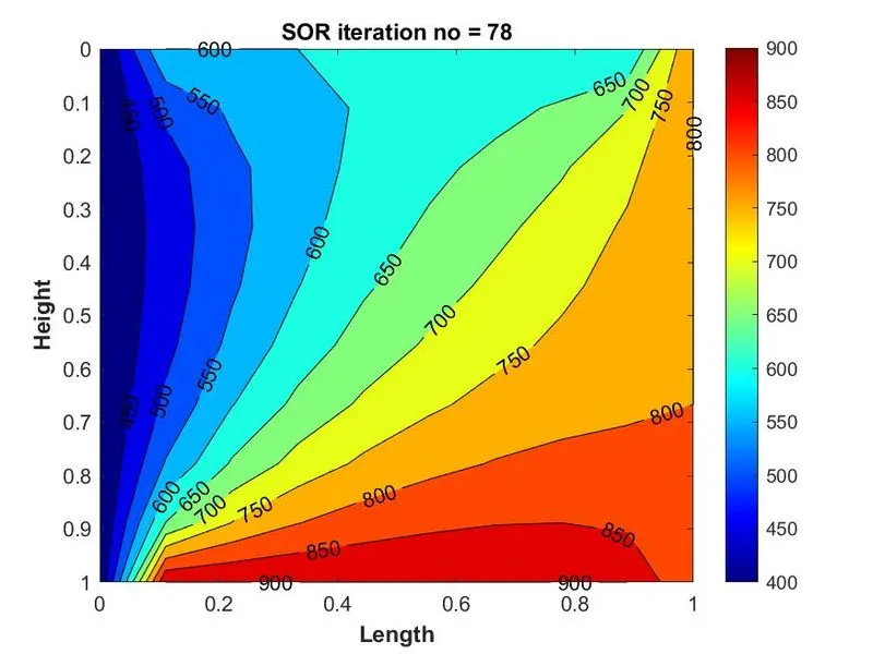
iii) Successive Over Relaxation Method:- The successive over-relaxation method is similar to the Gauss-Seidel method but it is based on a scaling factor or acceleration parameter w(omega) which reduces error very fast.
Steady-state equation solution using Jacobi method in Matlab
clear all;
close all;
clc;

%inputs
iterative_solver = 1;

nx = 10;
ny = nx;
x = linspace(0,1,nx);
dx = x(2) - x(1);
y = linspace(0,1,ny);
dy = y(2) - y(1);

%time step
dt = 0.1;
t(1) = 0;
t(end) = 50;

T = ones(nx,ny);

%applying boundary condition
T(1,:) = 600; %Top
T(nx,:) = 900; %Bottom
T(:,1) = 400; %left
T(:,ny) = 800; %right

k = 2*((dx^2+dy^2)/((dx^2)*(dy^2)));

Told = T;

error = 1e-2;
tol = 1e-4;

    %jacobi method
    if iterative_solver == 1
        jacobi_iter = 1;
        while(error > tol)
            for i = 2:nx-1
                for j = 2:ny-1
                    T(i,j) = (Told(i-1,j) + Told(i+1,j))/(k*dx^2) + (Told(i,j-1) + Told(i,j+1))/(k*dy^2);
                end
            end

            error = max(max(abs(Told - T)));
            Told = T;
            jacobi_iter = jacobi_iter +1;
            contourf(x,y,T,'ShowText','on')
            colorbar;
            colormap(jet);
            ax = gca;
            ax.YDir = 'reverse';
            xlabel("Length",'fontweight','Bold')
            ylabel("Height",'fontweight','Bold')
            title_text = sprintf("Jacobi iteration no = %d",jacobi_iter);
            title(title_text)

        end
    end
output graph
Steady state equation solution using Gauss Seidal method
clear all;
close all;
clc;

%inputs
iterative_solver = 2;

nx = 10;
ny = nx;
x = linspace(0,1,nx);
dx = x(2) - x(1);
y = linspace(0,1,ny);
dy = y(2) - y(1);

alpha = 1.4; %thermal diffusitive

%time step
dt = 0.1;
t(1) = 0;
t(end) = 50;

T = ones(nx,ny);

%applying boundary condition
T(1,:) = 600; %Top
T(nx,:) = 900; %Bottom
T(:,1) = 400; %left
T(:,ny) = 800; %right

k = 2*((dx^2+dy^2)/((dx^2)*(dy^2)));

Told = T;
T_initial = T;

error = 1e-2;
tol = 1e-4;

    %jacobi method
    if iterative_solver == 2
        gs_iter = 1;
        while(error > tol)
            for i = 2:nx-1
                for j = 2:ny-1
                    T(i,j) = (T(i-1,j) + Told(i+1,j))/(k*dx^2) + (T(i,j-1) + Told(i,j+1))/(k*dy^2);
                end
            end

            error = max(max(abs(Told - T)));
            Told = T;
            gs_iter = gs_iter +1;
            contourf(x,y,T,'ShowText','on')
            colorbar;
            colormap(jet)
            ax = gca;
            ax.YDir = 'reverse';
            xlabel("Length",'fontweight','Bold')
            ylabel("Height",'fontweight','Bold')
            title_text = sprintf("Gauss Seidal iteration no = %d",gs_iter);
            title(title_text)

        end
    end
output graph
Steady state equation solution using Successive over Relaxation method
clear all;
close all;
clc;

%inputs
iterative_solver = 2;

nx = 10;
ny = nx;
x = linspace(0,1,nx);
dx = x(2) - x(1);
y = linspace(0,1,ny);
dy = y(2) - y(1);
womega = 1.2;

alpha = 1.4; %thermal diffusitive

%time step
dt = 0.1;
t(1) = 0;
t(end) = 50;

T = ones(nx,ny);

%applying boundary condition
T(1,:) = 600; %Top
T(nx,:) = 900; %Bottom
T(:,1) = 400; %left
T(:,ny) = 800; %right

k = 2*((dx^2+dy^2)/((dx^2)*(dy^2)));

Told = T;
T_initial = T;

error = 1e-2;
tol = 1e-4;

    %jacobi method
    if iterative_solver == 2
        sor_iter = 1;
        while(error > tol)
            for i = 2:nx-1
                for j = 2:ny-1
                    T(i,j) =(1-womega)*Told(i,j) + womega*((T(i-1,j) + Told(i+1,j))/(k*dx^2) + (T(i,j-1) + Told(i,j+1))/(k*dy^2));
                end
            end

            error = max(max(abs(Told - T)));
            Told = T;
            sor_iter = sor_iter +1;
            contourf(x,y,T,'ShowText','on')
            colorbar;
            colormap(jet)
            ax = gca;
            ax.YDir = 'reverse';
            xlabel("Length",'fontweight','Bold')
            ylabel("Height",'fontweight','Bold')
            title_text = sprintf("SOR iteration no = %d",sor_iter);
            title(title_text)
            pause(0.03)
        end
    end
output graph
B) Transient State Equation :-
2D transient heat conduction equation is
`(dT)/dt` = `α((d^2T)/(dx^2) + (d^2T)/(dy^2))`
`(T(i,j)^(n+1) – T(i,j)^n)/dt = α((T(i-1,j) – 2T(i,j) +T(i+1,j))/dx^2 + (T(i,j-1) – 2T(i,j) +T(i,j+1))/dy^2 )^((n) or (n+1))`
If power is n then it is explicit and if power is n+1 then it is inplicit. So when it is explicit then the equation is
`T(i,j)^(n+1) = T(i,j)^n + K1.(T(i-1,j) -2T(i,j) + T(i+1,j))^n + K2.(T(i,j-1) -2T(i,j) + T(i,j+1))^n`
where k1 = `α(dt/dx^2)` and k2 =`α(dt/dy^2)` .In transient solution k1 = CFLx and k2 = CFLy and CFL = CFLx + CFLy = k1 + k2
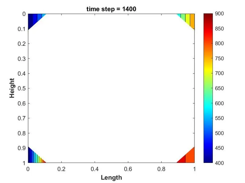
In explicit diffusion problem CFL<= 0.5 and if dx = dy then k1 = k2 <= 0.25. If CFL value greater than 0.5 the solution will be unstable.
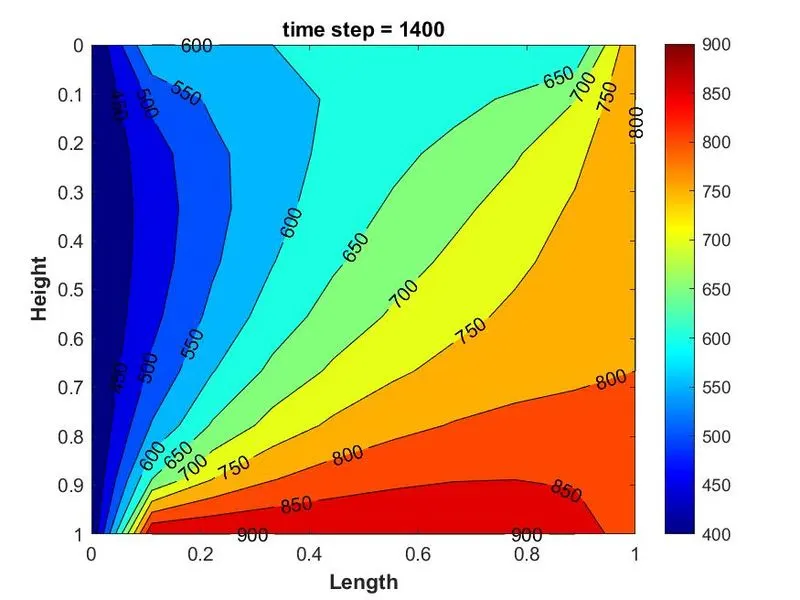
We can't use the iteration method in the explicit heat conduction equation. The solution of explicit heat conduction equation in Matlab
clear all;
close all;
clc;

%inputs

nx = 10;
ny = nx;
x = linspace(0,1,nx);
dx = x(2) - x(1);
y = linspace(0,1,ny);
dy = y(2) - y(1);

alpha = 1.4; %thermal diffusitive

%time step
dt = 0.001;
t(1) = 0;
t(end) = 50;

T = ones(nx,ny);

%applying boundary condition
T(1,:) = 600; %Top
T(nx,:) = 900; %Bottom
T(:,1) = 400; %left
T(:,ny) = 800; %right

k1 = alpha*(dt/dx^2);
k2 = alpha*(dt/dy^2);

%CFL <= 0.5
%CFL = k1 + k2 <= 0.5
cfl = k1 + k2;

% keeping a copy of T
Told = T;

for nt = 1:1400
    for i = 2:nx-1
        for j = 2:ny-1
            T(i,j) = Told(i,j) + k1*(Told(i-1,j) - 2*Told(i,j) + Told(i+1,j)) + k2*(Told(i,j-1) - 2*Told(i,j) + Told(i,j+1));
        end
    end
    Told = T;
end
contourf(x,y,T,'ShowText','on');
colorbar;
colormap(jet);
ax = gca;
ax.YDir = 'reverse';
xlabel("Length",'fontweight','Bold')
ylabel("Height",'fontweight','Bold')
title_text = sprintf("time step = %d",nt);
title(title_text)
output graph
If CFL is greater than 0.5 then the solution will be unstable and this matlab programme shows this
clear all;
close all;
clc;

%inputs

nx = 10;
ny = nx;
x = linspace(0,1,nx);
dx = x(2) - x(1);
y = linspace(0,1,ny);
dy = y(2) - y(1);

alpha = 1.4; %thermal diffusitive

%time step
dt = 0.1;
t(1) = 0;
t(end) = 50;

T = ones(nx,ny);

%applying boundary condition
T(1,:) = 600; %Top
T(nx,:) = 900; %Bottom
T(:,1) = 400; %left
T(:,ny) = 800; %right

k1 = alpha*(dt/dx^2);
k2 = alpha*(dt/dy^2);

%CFL <= 0.5
%CFL = k1 + k2 <= 0.5
cfl = k1 + k2;

% keeping a copy of T
Told = T;

for nt = 1:1400
    for i = 2:nx-1
        for j = 2:ny-1
            T(i,j) = Told(i,j) + k1*(Told(i-1,j) - 2*Told(i,j) + Told(i+1,j)) + k2*(Told(i,j-1) - 2*Told(i,j) + Told(i,j+1));
        end
    end
    Told = T;
end
contourf(x,y,T,'ShowText','on');
colorbar;
colormap(jet);
ax = gca;
ax.YDir = 'reverse';
xlabel("Length",'fontweight','Bold')
ylabel("Height",'fontweight','Bold')
title_text = sprintf("time step = %d",nt);
title(title_text)
print("explicit figure","-djpeg")
output graph
So now implicit heat conduction equation
`T(i,j)^(n+1) = (1/(1+2k1+2k2))[T(i,j)^n + K1.(T(i-1,j) + T(i+1,j))^(n+1) + K2.(T(i,j-1) + T(i,j+1))^(n+1)]`
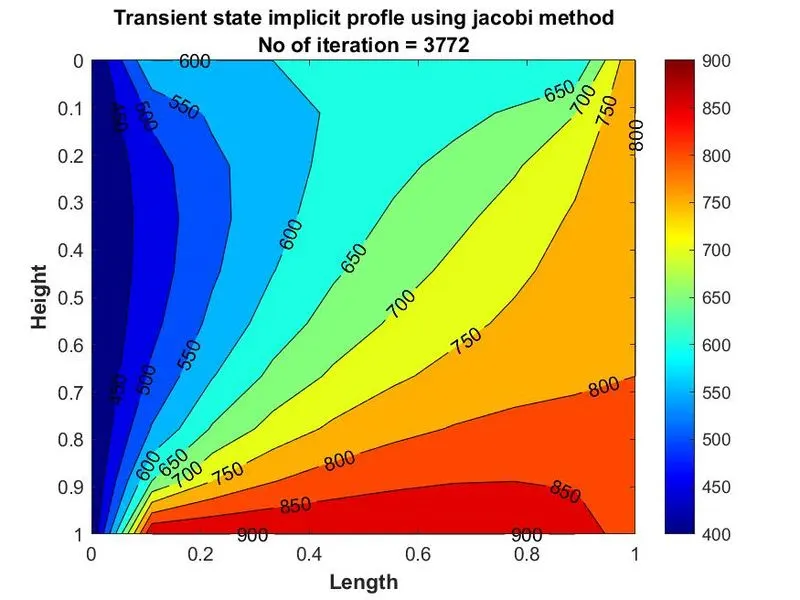
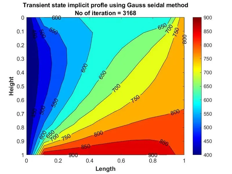
here also K1 = `α(dt/dx^2)` and K2 = `α(dt/dy^2)` and but in case of implicit only for the big value of CFL like 100 we see the changes in solution, the solution will be unstable. In the case of the implicit heat conduction equation, we use the three iterative methods i) Jacobi method ii) Gauss seidel method iii) Successive over relaxation method for getting the solution.
Implicit heat conduction equation solution using Jacobi iteration method:-
%Transient heat conduction equation dT/dt = alpha*(d^2T/dx^2 + d^2T/dy^2)
%this implicit equation solved by Gauss Seidal method

clear all;
close all;
clc;

%inputs
iterative_solver = 1;

nx = 10;
ny = nx;
x = linspace(0,1,nx);
dx = x(2) - x(1);
y = linspace(0,1,ny);
dy = y(2) - y(1);

alpha = 1.6; %thermal diffusitive

%time step
dt = 0.001;
t(1) = 0;
t(end) = 50;

T = ones(nx,ny);

%applying boundary condition
T(1,:) = 600; %Top
T(nx,:) = 900; %Bottom
T(:,1) = 400; %left
T(:,ny) = 800; %right

k1 = alpha*(dt/dx^2);
k2 = alpha*(dt/dy^2);

%CFL = CFL(x) + CFL(y) = k1 + k2
cfl = k1 + k2;

Told = T;
T_prev_dt = T;

error = 9e9;
tol = 1e-4;

    %jacobi method
    if iterative_solver == 1
        jacobi_iter = 1;
        for nt = 1:1400
            error = 9e9;
            while(error > tol)
                for i = 2:nx-1
                    for j = 2:ny-1
                        term1 = (1 + 2*k1 + 2*k2)^-1;
                        term2 = k1*term1;
                        term3 = k2*term1;
                        H = (Told(i-1,j) + Told(i+1,j));
                        V = (Told(i,j-1) + Told(i,j+1));
                        T(i,j) = (T_prev_dt(i,j)*term1) + (H*term2) + (V*term3);
                    end
                end

                error = max(max(abs(Told - T)));
                Told = T;
                jacobi_iter = jacobi_iter +1;

            end
            T_prev_dt = T;

        end

    end
    [c,h] = contourf(x,y,T,'ShowText','on');
    clabel(c,h)
    colorbar;
    colormap(jet)
    ax = gca;
    ax.YDir = 'reverse';
    xlabel("Length",'fontweight','Bold')
    ylabel("Height",'fontweight','Bold')
    title({'Transient state implicit profle using jacobi method'; ['No of iteration = ',num2str(jacobi_iter)]})
output graph
Transient implicit heat conduction equation solution using Gauss seidal method:-
%Transient heat conduction equation dT/dt = alpha*(d^2T/dx^2 + d^2T/dy^2)
%this implicit equation solved by Gauss Seidal method

clear all;
close all;
clc;

%inputs
iterative_solver = 2;

nx = 10;
ny = nx;
x = linspace(0,1,nx);
dx = x(2) - x(1);
y = linspace(0,1,ny);
dy = y(2) - y(1);

alpha = 1.6; %thermal diffusitive

%time step
dt = 0.001;
t(1) = 0;
t(end) = 50;

T = ones(nx,ny);

%applying boundary condition
T(1,:) = 600; %Top
T(nx,:) = 900; %Bottom
T(:,1) = 400; %left
T(:,ny) = 800; %right

k1 = alpha*(dt/dx^2);
k2 = alpha*(dt/dy^2);

%CFL = CFL(x) + CFL(y) = k1 + k2
cfl = k1 + k2;

Told = T;
T_prev_dt = T;

error = 9e9;
tol = 1e-4;

    %jacobi method
    if iterative_solver == 2
        gs_iter = 1;
        for nt = 1:1400
            error = 9e9;
            while(error > tol)
                for i = 2:nx-1
                    for j = 2:ny-1
                        term1 = (1 + 2*k1 + 2*k2)^-1;
                        term2 = k1*term1;
                        term3 = k2*term1;
                        H = (T(i-1,j) + Told(i+1,j));
                        V = (T(i,j-1) + Told(i,j+1));
                        T(i,j) = (T_prev_dt(i,j)*term1) + (H*term2) + (V*term3);
                    end
                end

                error = max(max(abs(Told - T)));
                Told = T;
                gs_iter = gs_iter +1;

            end
            T_prev_dt = T;

        end

    end
    [c,h] = contourf(x,y,T,'ShowText','on');
    clabel(c,h)
    colorbar;
    colormap(jet)
    ax = gca;
    ax.YDir = 'reverse';
    xlabel("Length",'fontweight','Bold')
    ylabel("Height",'fontweight','Bold')
    title({'Transient state implicit profle using Gauss seidal method'; ['No of iteration = ',num2str(gs_iter)]})
output graph
Transient heat conduction equation solution using Successive over relaxation method:-
%Transient heat conduction equation dT/dt = alpha*(d^2T/dx^2 + d^2T/dy^2)
%this implicit equation solved by Successive Over relaxation method

clear all;
close all;
clc;

%inputs
iterative_solver = 2;

nx = 10;
ny = nx;
x = linspace(0,1,nx);
dx = x(2) - x(1);
y = linspace(0,1,ny);
dy = y(2) - y(1);

alpha = 1.6; %thermal diffusitive

%time step
dt = 0.001;
t(1) = 0;
t(end) = 50;

T = ones(nx,ny);

%applying boundary condition
T(1,:) = 600; %Top
T(nx,:) = 900; %Bottom
T(:,1) = 400; %left
T(:,ny) = 800; %right

k1 = alpha*(dt/dx^2);
k2 = alpha*(dt/dy^2);

%CFL = CFL(x) + CFL(y) = k1 + k2
CFL = k1 + k2;

womega = 1.1;

Told = T;
T_prev_dt = T;

error = 9e9;
tol = 1e-4;

%jacobi method
if iterative_solver == 2
   sor_iter = 1;
   for nt = 1:1400
       error = 9e9;
       while(error > tol)
             for i = 2:nx-1
                 for j = 2:ny-1
                     term1 = (1 + 2*k1 + 2*k2)^-1;
                     term2 = k1*term1;
                     term3 = k2*term1;
                     H = (T(i-1,j) + Told(i+1,j));
                     V = (T(i,j-1) + Told(i,j+1));
                     T(i,j) = (T_prev_dt(i,j)*term1) + (H*term2) + (V*term3);
                     T(i,j) = (1 - womega)*Told(i,j) + womega*(T(i,j));
                 end
             end

             error = max(max(abs(Told - T)));
             Told = T;
             sor_iter = sor_iter +1;

        end
            T_prev_dt = T;

    end

end
[c,h] = contourf(x,y,T,'ShowText','on');
clabel(c,h)
colorbar;
colormap(jet)
ax = gca;
ax.YDir = 'reverse';
xlabel("Length",'fontweight','Bold')
ylabel("Height",'fontweight','Bold')
title({'Transient state implicit profle using Successive Over Relaxation method'; ['No of iteration = ',num2str(sor_iter)]})
output graph
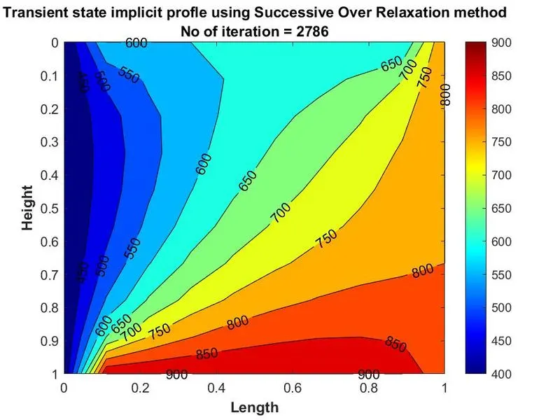
In transient heat conduction equation for explicit is taken very little time to converge the solution but implicit take greater time than an explicit approach to converge but the implicit approach is greater stable than explicit approach because here we use iteration method. And among the three iterative methods Successive Over Relaxation method reduces the error very quickly and converges the solution.