Week 3.5 - Deriving 4th order approximation of a 2nd order derivative using Taylor Table method

AIM:-The project aims to derive the Central difference, Skewed right-sided difference, and Skewed left-sided difference scheme for the fourth-order approximation of second-order derivative. We find here which scheme’s error is lesser and also we know from this project why we use skewed scheme.

JOB REPORT :- Here we pick up a function f(x) = exp(x)*cos(x)

CENTRAL DIFFERENCE SCHEME :- For deriving the central difference scheme for fourth order approximation of 2^nd order derivative by Taylor table method of finite difference method we know,

No of nodes = p + q - 1 [where, p = order of derivation and q = order of

approximation]

= 2 + 4 - 1 = 5

So the equation is

`(d^2f(x)) /dx^2 = (a f(x – 2dx) + b f(x-dx) + c f(x) + d f(x+dx) + e f(x+2dx))/(dx^2)`

The co-efficient a, b, c, d and e are computed by Taylor’s Table :-

`(d^2f(x)) /(dx^2)`	f(x)	dx f’(x)	dx2 f’’(x)	dx3 f’’’(x)	dx4 f’’’’(x)
a f(x – 2dx)	a	-2a	2a	`-(8a)/6`	`(16a)/24`
b f(x-dx)	b	-b	`b/2`	-b/6	b/24
c f(x)	c	0	0	0	0
d f(x+dx)	d	d	`d/2`	`d/6`	`d/24`
e f(x+2dx)	e	2e	2e	`(8e)/6`	`(16e)/24`
Total	0	0	1	0	0

So from this Taylor’s table we get 5 algebraic equation

a + b + c + d + e = 0

-2a – b + d + 2e = 0

4a + b + d + d +4e = 2

-8a - b + d + 8e = 0

16a + b + d + 16e = 0

So from these 5 equation we get these 5 equation value

a = - 0.0833

b = 1.3333

c = -2.500

d = 1.3333

e = - 0.0833

So if f(x) = exp(x)*cos(x) then

u

`(d^2f(x)) /(dx^2) = (- 0.0833exp(x-2dx)cos(x-2dx) + 1.3333exp(x-dx)cos(x-dx) - 2.5exp(x)cos(x) + 1.3333exp(x+dx)cos(x+dx) -0.0833exp(x+2dx)cos(x+2dx))/(dx^2)`

SKEWED RIGHT SIDE DIFFERENCE :- For deriving the skewed right side difference for fourth order approximation of 2^nd order derivative by Taylor table method of finite difference method we know,

No of nodes = p + q [where, p = order of derivation and q = order of

approximation]

= 2 +4 = 6

So the equation is

`(d^2f(x))/(dx^2) = (a f(x) + b f(x+1dx) + c f(x+2dx) + d f(x+3dx) + e f(x+4dx) + g f(x+5dx))/(dx2)`

The co-efficient a, b, c, d, e and g are computed by Taylor’s Table :-

`(d^2f(x))/dx^2`	f(x)	dx f’(x)	dx2 f’’(x)	dx3f’’’(x)	dx3 f’’’’(x)	dx4 f’’’’’(x)
af(x)	a	0	0	0	0	0
b f(x+1dx)	b	b	`b/2`	`b/6`	`b/24`	`b/120`
c f(x+2dx)	c	2c	`(4c)/2`	`(8c)/6`	`(16c)/24`	`(32c)/120`
d f(x+3dx)	d	3d	`(9d)/2`	`(27d)/6`	`81d/24`	`(243d)/120`
e f(x+4dx)	e	4c	`(16e)/2`	`(64e)/6`	`(256e)/24`	`(1024e)/120`
g f(x +5dx)	g	5g	`(25g)/2`	`(125g)/6`	`(625g)/24`	`(3125g)/120`
Total	0	0	1	0	0	0

From this Taylor’s Table we get 6 algebraic equation

a + b + c + d + e + g = 0……..(i)

b + 2c + 3d + 4c + 5g = 0……(ii)

`b/2 + (4c)/2 +(9d)/2 + (16e)/2 +(25g)/2 = 1`……..(iii)

`b/6 + (8c)/6 + (27d)/6 + (64e)/6 + (125g)/6 = 0`……..(iv)

`b/24 + (16c)/24 + (81d)/24 +( 256e)/24 + ( 625g)/24 = 0`…….(v)

`b/120 + (32c)/120 + (243d)/120 + (1024e)/120 + (3125g)/120 = 0`…….(vi)

from this 6 equation we get the value of

a = 3.75

b = -12.833

c = 17.833

d = -13

e = 5.0833

g = - 0.8333

So if f(x) = exp(x)*cos(x) then

`(d^2f(x)) /(dx^2) = (3.75*exp(x)*cos(x) - 12.833 *exp(x+1dx) *cos(x+dx) + 17.833*exp(x+2dx) *cos(x+2dx) – 13 *exp(x+3dx) *cos(x+3dx) + 5.0833* exp(x+4dx) *cos(x+4dx) - 0.833 *exp(x+5dx) *cos(x+5dx))/(dx^2)`

SKEWED LEFT SIDE DIFFERENCE :- For deriving the skewed left side difference for fourth order approximation of 2^nd order derivative by Taylor table method of finite difference method we know,

No of nodes = p + q [where, p = order of derivation and q = order of

approximation]

= 2 +4 = 6

So the equation is

`(d^2f(x))/(dx^2) = (a f(x) + b f(x-dx) + c f(x-2dx) + d f(x-3dx) + e f(x-4dx) + g f(x-5dx))/(dx^2)`

The co-efficient a, b, c, d, e and g are computed by Taylor’s Table :-

d2f(x)/dx2	f(x)	dx f’(x)	dx2 f’’(x)	dx3f’’’(x)	dx3 f’’’’(x)	dx4 f’’’’’(x)
af(x)	a	0	0	0	0	0
b f(x-1dx)	b	-b	b/2	-b/6	b/24	-b/120
c f(x-2dx)	c	-2c	4c/2	-8c/6	16c/24	-32c/120
d f(x-3dx)	d	-3d	9d/2	-27d/6	81d/24	-243d/120
e f(x-4dx)	e	-4c	16e/2	-64e/6	256e/24	-1024e/120
g f(x -5dx)	g	-5g	25g/2	-125g/6	625g/24	-3125g/120
Total	0	0	1	0	0	0

From this Taylor’s Table we get 6 algebraic equation

a + b + c + d + e + g = 0……..(i)

b + 2c + 3d + 4c + 5g = 0……(ii)

b/2 + 4c/2 +9d/2 + 16e/2 +25g/2 = 1……..(iii)

b/6 + 8c/6 + 27d/6 + 64e/6 + 125g/6 = 0……..(iv)

b/24 + 16c/24 + 81d/24 + 256e/24 + 625g/24 = 0…….(v)

b/120 + 32c/120 + 243d/120 + 1024e/120 + 3125g/120 = 0…….(vi)

from this 6 equation we get the value of

a = 3.75

b = -12.833

c = 17.833

d = -13

e = 5.0833

g = - 0.8333

So if f(x) = exp(x)*cos(x) then

d²f(x) /dx² = (3.75exp(x) cos(x) - 12.833exp(x-dx)*cos(x-dx) + 17.8333exp(x-2dx) cos(x-2dx) - 13exp(x-3dx) cos(x-3dx) + 5.0833exp(x-4dx) cos(x-4dx) - 0.8333exp(x-5dx) cos(x-5dx))/(dx^2)

POGRAMME ON MATLAB :-

First create the function of Central Difference Scheme in Matlab

function error1 = cds_error(x,dx)
 %f(x) = exp(x)*cos(x)
 %analytical derivative
 %f'(x) = exp(x)*cos(x) - exp(x)*sin(x)
 %f''(x) = - 2*exp(x)*sin(x)
 analytical_derivative = - 2*exp(x)*sin(x);
 
 % numerical derivative
 c_approximation = (- 0.0833*exp(x-(2*dx))*cos(x-(2*dx)) + 1.3333*exp(x-dx)*cos(x-dx) - 2.5*exp(x)*cos(x) + 1.3333*exp(x+dx)*cos(x+dx) - 0.0833*exp(x+(2*dx))*cos(x+(2*dx)))/(dx^2);
 
 error1 = abs(analytical_derivative - c_approximation);
 
end

Secondly we create the functionb of Skewed Right side scheme

function error2 = RSS_error(x,dx)

 %f'(x) = exp(x)*cos(x) - exp(x)*sin(x)
 %f''(x) = - 2*exp(x)*sin(x)
 %analytical derivative
 analytical_derivative = - 2*exp(x)*sin(x);
 
%numerical derivative
RSS_approximation = (3.75*exp(x)*cos(x) - 12.833*exp(x+dx)*cos(x+dx) + 17.833*exp(x+(2*dx))*cos(x+(2*dx)) - 13*exp(x+(3*dx))*cos(x+(3*dx)) + 5.0833*exp(x+(4*dx))*cos(x+(4*dx)) - 0.833*exp(x+(5*dx))*cos(x+(5*dx)))/(dx^2);

error2 = abs(analytical_derivative - RSS_approximation);

end

thirdly we create the function of Skewed Left side scheme

function error3 = LSS_error(x,dx)
%f(x) = exp(x)*cos(x)
%f'(x) = exp(x)*cos(x) - exp(x)*sin(x)
 %f''(x) = - 2*exp(x)*sin(x)
 %analytical derivative
 analytical_derivative = - 2*exp(x)*sin(x);
 
 % numerical derivative
 LSS_approximation = (3.75*exp(x)*cos(x) - 12.833*exp(x-dx)*cos(x-dx) + 17.8333*exp(x-(2*dx))*cos(x-(2*dx)) - 13*exp(x-(3*dx))*cos(x-(3*dx)) + 5.0833*exp(x-(4*dx))*cos(x-(4*dx)) - 0.8333*exp(x-(5*dx))*cos(x-(5*dx)))/(dx^2);
 
 error3 = abs(analytical_derivative - LSS_approximation);

end

Now we create Forward differencing Approximation function and Backward differencing Approximation function scheme which we previously learn

Forward differencing Approximation

function error4 = forward_difference_scheme(x,dx)
%f(x) = exp(x)*cos(x)
%Analytical derivative 
analytical_derivative = - 2*exp(x)*sin(x);

%numerical derivative
f_differencing = (exp(x)*cos(x) - 2*exp(x+dx)*cos(x+dx) + exp(x+(2*dx))*cos(x+(2*dx)))/(dx^2);

error4 = abs(analytical_derivative - f_differencing);
end

Backward differencing Approximation

function error5 = backward_difference_scheme(x,dx)
%f(x) = exp(x)*cos(x)
%Analytical derivative 
analytical_derivative = - 2*exp(x)*sin(x);

%numerical derivative
b_differencing = (exp(x+2*dx)*cos(x+2*dx) - 2*exp(x+dx)*cos(x+dx) + exp(x)*cos(x))/(dx^2);

error5 = abs(analytical_derivative - b_differencing);
end

Now the main programme

clear all;
close all;
clc;
x = 2*pi;
dx = linspace(pi/4,pi/400000,200);

for i = 1:length(dx)
    
    skewed_LSS_error(i) = LSS_error(x,dx(i));
    skewed_RSS_error(i) = RSS_error(x,dx(i));
    centra_differencing_scheme(i) = cds_error(x,dx(i));
    f_diff_scheme_error(i) = forward_difference_scheme(x,dx(i));
    b_diff_scheme_error(i) = backward_difference_scheme(x,dx(i));
    
end

figure(1)
loglog(dx,skewed_LSS_error,'b','marker','D')
hold on;
loglog(dx,skewed_RSS_error,'k','marker','s')
hold on;
loglog(dx,centra_differencing_scheme,'r','marker','o')
hold on;
loglog(dx,f_diff_scheme_error,'y','marker','*')
hold on;
loglog(dx, b_diff_scheme_error,'g')
hold off;
xlabel("dx")
ylabel("Error")
legend("skewed left side error", "skewed right side error", "central differencing error", "forward differencing error","backward differencing error")

output:-

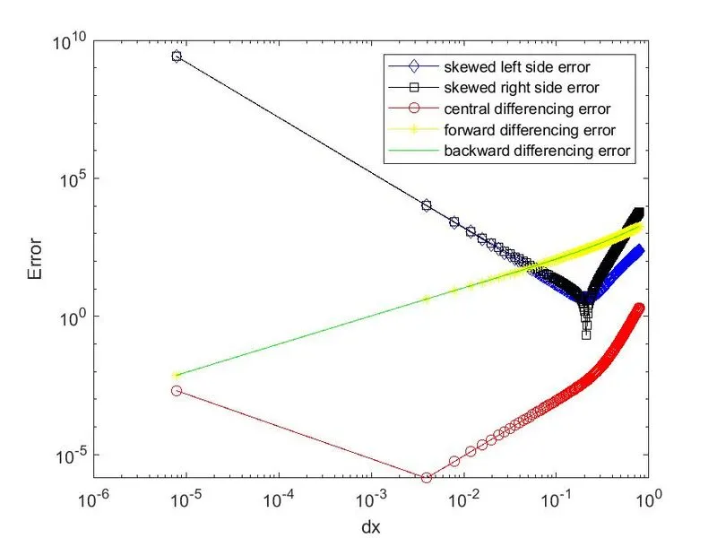
The resulting graph is

CONCLUSION :-

From the above graph we can see that the central difference approximation more accurate than the right skewed and left skewed scheme . Since forward and backward difference scheme error is increasing constantly with the increasing of dx.

In the range dx of 10^-6 to 10^-2 the error is very high for right skewed and left skewed scheme but in range 10^-2 to 1 error is low compare to the forward and backward difference scheme and then again error rises . In range of 10^-6 to 10^-2 the central difference scheme’s error is decreasing with the increase of dx and after that error rises.

Why skewed scheme is necessary though central difference scheme is greater ?

A function is always characterized by a domain. A domain is a area beyond which a function ceases to exit. In order to apply the approximation scheme at boundaries, only skewed scheme is applicable. While due to the unavailability of grid points on one of the sides of boundary, the central scheme can’t be applied. Because it requires a number of grid points on both sides of the reference points depending upon the order of approximation scheme and order of derivative to be evaluated.