Week 7 - Simulation of a 1D Super-sonic nozzle flow simulation using Macormack Method
AIM:- The project aims is to simulate the isentropic flow through a quasi 1D subsonic–supersonic nozzle. We derive both conservation and non-conservation forms of governing equations and we are comparing both the form of governing equations by comparing their solution.
OBJECTIVE:- Here our main objective is the comparison between conservation and non-conservation forms of governing equations. We solve those governing equations using MacCormack's technique. We need to determine the steady-state temperature distribution for the flow-field variables and investigate the difference between the two forms of governing equations by comparing their solutions.
In this project, we see
1. Steady-state distribution of primitive variables inside the nozzle
2. Time-wise variation of the primitive variables
3. Variation of Mass flow rate distribution inside the nozzle at different time steps during the time-marching process
4. Comparison of Normalized mass flow rate distributions of both forms
PROJECT REPORT:- We consider the steady, isentropic flow through a convergent-divergent nozzle. The flow at the inlet to the nozzle comes from a reservoir where the pressure and temperature are denoted by `P_0` and `T_0`, respectively. The cross-sectional area of the reservoir is very large (theoretically, A `rarr ∞` ), and hence the velocity is very small (v`rarr 0` ).Thus p0 and T0 are stagnation values, or total pressure and total temperature, respectively. The flow expands isentropically to supersonic speeds at the nozzle exit, where the exit pressure, temperature, velocity, and Match number are denoted by pe, Te, ve, and Me, respectively. The flow is locally subsonic in the convergent section of the nozzle and sonic at the throat section(minimum area) and supersonic at the divergent section.
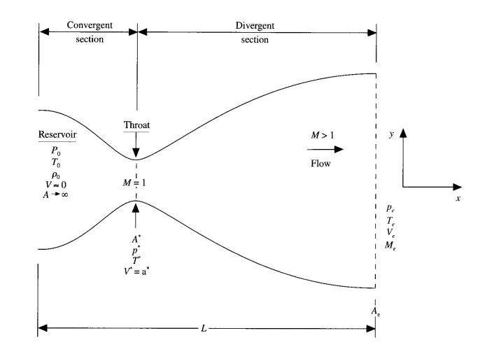
The governing continuity, momentum, energy equation for a quasi-one-dimensional, steady, isentropic flow can be expressed as
Continuity: `ρ_1 V_1 A_1 = ρ_2 V_2 A_2`
Momentum: `p_1 A_1+ρ_1 V_1^2 A_1+∫_(A_1)^(A_2)p dA = p_2 A_2 + ρ_2 V_2^2 A_2`
Energy: `h_1 + (V_1^2)/2 = h_2 + (V_2^2)/2`
In reality, the nozzle flow is two-dimensional because with the area changing as a function of x, actually there will be flow field variation in both x and y directions. This is the real physics of flow and the equation properly describes two-dimensional flow but the equation which satisfies the real physics does not properly satisfy the quasi-one-dimensional flow. To ensure all physical principles are satisfied, we apply an integral form of governing equation to a control volume consistent with quasi-one-dimensional assumption.
We apply the integral form of governing equation to the shaded control volume. This control volume is a slice of the nozzle flow, where the infinitesimal thickness of the slice is dx.
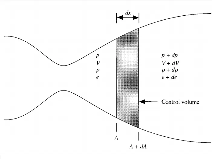
On the left side of the control volume, consistent with the quasi-one-dimensional assumption, the density, velocity, pressure, and internal energy, denoted by `ρ`, V, p, e, respectively are uniform over area A. Similarly, on the right side of the control volume, the density, velocity, pressure, and internal energy, denoted by `ρ+dρ`, V + dV, p + dp, e + de, respectively are uniform over the area A+dA.
Solving the integral form of governing equations we get two types of governing equations. One is the Conservative form and another is the Non-conservative form.
Conservative form
Continuity equation:
`(∂(ρ^' A^' ))/(∂t^' )+ (∂(ρ^' A^' V^' ))/(∂x^' )=0`
Momentum equation:
`(∂(ρ^' A^' V'))/(∂t^' )+ (∂[ρ^' A^' (V^')^(2 )+ (1/γ)ρ^' A^'])/(∂x^' )= (1/γ)(ρ^' (∂A^')/(∂x^'))`
Energy equation:
`(∂[ρ'((e^')/(γ-1) + γ/2 (V^')^2 )A'])/(∂t')+ (∂[ρ^' (e^'/(γ-1)+ γ/2 (V^')^2 ) V^' A^' + ρ'A'V'])/(∂x^')=0`
Non-Conservative form
Continuity equation:
`(∂ρ^')/(∂t^' )= -ρ^' (∂V^')/(∂x^' )- ρ^' V^' (∂(lnA^' ))/(∂x^' )-V'(∂ρ^')/(∂x^' )`
Momentum equation:
`(∂V^')/(∂t^')= -V^' (∂V^')/(∂x^') - 1/γ((∂T^')/(∂x^')+(T^')/(ρ^') (∂ρ^')/(∂x^'))`
Energy equation
`(∂T^')/(∂t^' )= V^' (∂T^')/(∂x^' )-(γ-1) T^' [(∂V^')/(∂x^' )+V'(∂(lnA'))/(∂x^' )]`
Non-Dimensional Properties
Non-Dimensional Density, `ρ^'= ρ/ρ_0`
Non-Dimensional Temperature, `T^' = T/T_0`
Non-Dimensional distance,`V^' = V/a_0`[Here `a_0` is the local sonic velocity and `a_0` = `√(γRT_0)` ]
Non-Dimensional area, `A^' = A/A_0`
Non-Dimensional time, `t^' = t/(L/a_0)`
MACCORMACK TECHNIQUE:
MacCormack method is an explicit finite difference technique that is second-order accurate in both space and time. It is one of the popular explicit finite difference methods for solving fluid flow problems. It is student-friendly, easiest and the result obtained by using this technique are perfectly satisfactory for many fluid flow applications. That’s why we use this technique to solve the Conservative form and Non-Conservative form of the governing equation. To solve the quasi-one-dimensional subsonic-supersonic nozzle fluid flow problem it has two parts Predictor step and Corrector step. But, first of all, we have to define all the initial values and then we go for a solution.
- Predictor Step:- In the continuity equation, we replace the spatial derivatives on the right-hand side with forward differences. In the equation, all flow variables at time t are known values. So the right-hand side is known. Now a predicted value of a primitive variable, (primitive variable)^(t+ t), from the first two terms of the Taylor series. So after this step, we update all the primitive variables.
`((df)/(dt) )_p= (f_(i+1)- f_i)/dt`
And updating the variable
`f_(p )= f_(Initial)+ ((df)/(dt) )_p`
- Corrector Step:- In the corrector step, we first obtain predicted values of the time derivative at a time (t+ t), by substituting the predicted values of U, and v into the right side of the continuity equation, replacing the spatial derivatives with reward difference.
Now we have to do the average of the corrector value and predicted value.
`((df)/(dt) )_c= (f_i- f_(i-1))/dt`
and
`((df)/(dt) )_(avg)= {((df)/(dt)) _p + ((df)/(dt)) _c }`
And then we update the final solution
`f_(s )= f_(Initial )+ ((df)/(dt) )_(avg)`
Now the main code
clear all;
close all;
clc;

n = 31;
x = linspace(0,3,n);
gamma = 1.4;

%time steps
nt = 1400;

%corant number
C = 0.5;

% %Non_conservative equation
[A_nc,roh_nc,T_nc,v_nc,P_nc,Mfr_nc,Match_number_nc,MFR_throat_nc] = non_conservation_equation(x,n,C,nt,gamma);

%The plot between Primitive variables and flow rate distribution
figure(1)

subplot(5,2,1)
plot(x,A_nc,'color','b','LineWidth',1.5)
hold on;
plot(x,(-A_nc),'color','b','LineWidth',1.5)
hold on;
plot([x(16) x(16)],[-5 5],'--','color','k')
xlabel("Nozzle length","FontWeight","Bold")
ylabel("Area","FontWeight","Bold")
axis([0 3 -10 10])
hold off;

subplot(5,2,3)
plot(x,P_nc,'color','c','LineWidth',1.5)
hold on;
plot([0 x(16)], [P_nc(16) P_nc(16)], '--','color','k')
hold on;
plot([x(16) x(16)], [0 P_nc(16)], '--','color','k')
hold on;
plot([0 x(30)], [P_nc(31) P_nc(31)], '--', 'color','k')
xlabel("Nozzle length","FontWeight","Bold")
ylabel("Pressure","FontWeight","Bold")
yticks([0 P_nc(31) P_nc(16) 1])
yticklabels({'0','P_e/P_o',P_nc(16),'1'})
axis([0 3 0 1])
hold off;

subplot(5,2,4)
plot(x,T_nc,'color','m','LineWidth',1.5)
hold on;
plot([0 x(16)], [T_nc(16) T_nc(16)], '--','color','k')
hold on;
plot([x(16) x(16)], [0 T_nc(16)], '--','color','k')
hold on;
plot([0 x(30)], [T_nc(31) T_nc(31)], '--', 'color','k')
xlabel("Nozzle length","FontWeight","Bold")
ylabel("Temperature","FontWeight","Bold")
yticks([0 T_nc(31) T_nc(16) 1])
yticklabels({'0','T_e/T_o',T_nc(16),'1'})
axis([0 3 0 1])
hold off;

subplot(5,2,5)
plot(x,roh_nc,'color','r','LineWidth',1.5)
hold on;
plot([0 x(16)], [roh_nc(16) roh_nc(16)], '--','color','k')
hold on;
plot([x(16) x(16)], [0 roh_nc(16)], '--','color','k')
hold on;
plot([0 x(30)], [roh_nc(31) roh_nc(31)], '--', 'color','k')
xlabel("Nozzle length","FontWeight","Bold")
ylabel("Density","FontWeight","Bold")
yticks([0 roh_nc(31) roh_nc(16) 1])
yticklabels({'0','roh_e/roh_o',roh_nc(16),'1'})
axis([0 3 0 1])
hold off;

subplot(5,2,6)
plot(x,Match_number_nc,'color','g','LineWidth',1.5)
hold on;
plot([0 x(16)], [Match_number_nc(16) Match_number_nc(16)], '--','color','k')
hold on;
plot([x(16) x(16)], [0 Match_number_nc(16)], '--','color','k')
hold on;
plot([0 x(30)], [Match_number_nc(31) Match_number_nc(31)], '--', 'color','k')
ylabel("Match Number","FontWeight","Bold")
xlabel("Nozzle length","FontWeight","Bold")
yticks([0 1 Match_number_nc(31) 4])
yticklabels({'0',Match_number_nc(16),'M_e','4'})
axis([0 3 0 4])
hold off;

%Conservatrive equation
[A_c,roh_c,T_c,v_c,P_c,Mfr_c,Match_number_c,MFR_throat_c] = conservative_equation(x,n,C,nt,gamma);

%The plot between Primitive variables and flow rate distribution
figure(2)

subplot(5,2,1)
plot(x,A_c,'color','b','LineWidth',1.5)
hold on;
plot(x,(-A_c),'color','b','LineWidth',1.5)
hold on;
plot([x(16) x(16)],[-5 5],'--','color','k')
xlabel("Nozzle length","FontWeight","Bold")
ylabel("Area")
axis([0 3 -10 10])
hold off;

subplot(5,2,3)
plot(x,P_c,"linewidth",1.25,"color","m")
hold on;
plot([0 x(16)], [P_c(16) P_c(16)], '--','color','k')
hold on;
plot([x(16) x(16)], [0 P_c(16)], '--','color','k')
hold on;
plot([0 x(30)], [P_c(31) P_c(31)], '--', 'color','k')
xlabel("Nozzle length","FontWeight","Bold")
ylabel("Pressure","FontWeight","Bold")
yticks([0 P_nc(31) P_nc(16) 1])
yticklabels({'0','P_e/P_o',P_nc(16),'1'})
axis([0 3 0 1])
hold off;

subplot(5,2,4)
plot(x,T_c,"linewidth",1.25,"color","r")
hold on;
plot([0 x(16)], [T_c(16) T_c(16)], '--','color','k')
hold on;
plot([x(16) x(16)], [0 T_c(16)], '--','color','k')
hold on;
plot([0 x(30)], [T_c(31) T_c(31)], '--', 'color','k')
xlabel("Nozzle length","FontWeight","Bold")
ylabel("Temperature","FontWeight","Bold")
yticks([0 T_nc(31) T_nc(16) 1])
yticklabels({'0','T_e/T_o',T_nc(16),'1'})
axis([0 3 0 1])
hold off;

subplot(5,2,5)
plot(x,roh_c,"linewidth",1.25,"color","g")
hold on;
plot([0 x(16)], [roh_c(16) roh_c(16)], '--','color','k')
hold on;
plot([x(16) x(16)], [0 roh_c(16)], '--','color','k')
hold on;
plot([0 x(30)], [roh_c(31) roh_c(31)], '--', 'color','k')
xlabel("Nozzle length","FontWeight","Bold")
ylabel("Density","FontWeight","Bold")
yticks([0 roh_c(31) roh_c(16) 1])
yticklabels({'0','roh_e/roh_o',roh_c(16),'1'})
axis([0 3 0 1])
hold off;

subplot(5,2,6)
plot(x,Match_number_c,"linewidth",1.25,"color","y")
hold on;
plot([0 x(16)], [Match_number_c(16) Match_number_c(16)], '--','color','k')
hold on;
plot([x(16) x(16)], [0 Match_number_c(16)], '--','color','k')
hold on;
plot([0 x(30)], [Match_number_c(31) Match_number_c(31)], '--', 'color','k')
xlabel("Nozzle length","FontWeight","Bold")
ylabel("Match Number","FontWeight","Bold")
yticks([0 1 Match_number_c(31) 4])
yticklabels({'0',Match_number_c(16),'M_e','4'})
axis([0 3 0 4])
hold off;

%Comparision between the mass flow rate of conservation and
%non-conservation governing equation
figure(7);
plot(x,Mfr_nc,"linewidth",1.25,"color","m")
hold on;
plot(x,Mfr_c,"linewidth",1.25,"color","c")
xlabel("Nozzle length","FontWeight","Bold")
ylabel("Mass Flow Rate","FontWeight","Bold")
legend("Non-Conservation form","Conservation form","location","Best")
title(["Comparision between the mass flow rate of conservation and","non-conservation governing equations"])
hold off;

%Comparision between the mass flow rate of conservation and
%non-conservation governing equation in case of time step
figure(8);
plot(MFR_throat_nc,"linewidth",1.25,"color","m")
hold on;
plot(MFR_throat_c,"linewidth",1.25,"color","c")
xlabel("Time Step","FontWeight","Bold")
ylabel("Mass Flow Rate","FontWeight","Bold")
legend("Non-Conservation form","Conservation form","location","Best")
title(["Comparision between the mass flow rate of conservation and","non-conservation governing equations"])
hold off;

figs = findobj(0, 'type', 'figure');

for k=1:length(figs)
    % print each figure in figs to a separate .eps file
    print(figs(k), '-djpeg', sprintf('file%d.jpeg', k))
end
conservation equation
function [A_c,roh_c,T_c,v_c,P_c,Mfr_c,Match_number_c,MFR_throat_c] = conservative_equation(x,n,C,nt,gamma)

dx = x(2) - x(1);
%Nozzle Area
A = 1 + 2.2*((x - 1.5).^2);
throat = find(A == 1);

%Initial conditions
for i = 1:length(x)
    if ((x(i)>=0) && (x(i)<=0.5))
        roh(i) = 1;
        T(i) = 1;
    elseif((x(i)>=0.5) && (x(i)<=1.5))
        roh(i) = 1 - 0.366*(x(i) - 0.5);
        T(i) = 1 - 0.167*(x(i) - 0.5);
    elseif((x(i)>=1.5) && (x(i)<=3.5))
        roh(i) = 0.634 - 0.3879*(x(i) - 1.5);
        T(i) = 0.833 - 0.3507*(x(i) - 1.5);
    end
end

%Velocity and Pressure term
v = 0.59./(roh.*A); %
P = roh.*T;

a = (sqrt(T)); %local speed of sound
m_dot = roh.*A.*v;          %mass flow rate
M = v./a;                   %Match number

%Solution variable initialization
U1 = roh.*A ;
U2 = roh.*A.*v;
U3 = roh.*(T./(gamma - 1) + (gamma/2).*(v.^2)).*A;

for k = 1:nt
    %Copy of U1, U2, U3
    U1_old = U1;
    U2_old = U2;
    U3_old = U3;

    %Adaptive time step
    dt = min(C*dx./(a + v));

    for j = 2:n-1
        %Initialization of flux
        F1 = U2;
        F2 = (((U2).^2)./U1) + (((gamma - 1)/gamma).*(U3 - (gamma/2)*(U2.^2./U1)));
        F3 = (gamma).*((U2.*U3)./U1) - (gamma*(gamma -1))/2.*((U2.^3)./(U1.^2));
        %Source code
        J1(j) = (1/gamma).*roh(j).*T(j).*((A(j+1) - A(j))/dx);

        %The prediction step
        dU1_dt_p(j) = -(F1(j+1) - F1(j))/dx;
        dU2_dt_p(j) = -(F2(j+1) - F2(j))/dx + J1(j);
        dU3_dt_p(j) = -(F3(j+1) - F3(j))/dx;

        %Update the variable U1,U2 and U3
        U1(j) = U1(j) + dU1_dt_p(j)*dt;
        U2(j) = U2(j) + dU2_dt_p(j)*dt;
        U3(j) = U3(j) + dU3_dt_p(j)*dt;
    end

    %Update the density, temperature, velocity, pressure term
    roh = U1./A;
    v = U2./U1;
    T = (gamma-1).*(U3./U1 - (gamma/2).*v.^2);
    P = roh.*T;

    %Updation of flux
    F1 = U2;
    F2 = (((U2).^2)./U1) + (((gamma - 1)/gamma).*(U3 - (gamma/2)*(U2.^2./U1)));
    F3 = (gamma).*((U2.*U3)./U1) - (gamma*(gamma -1))/2.*((U2.^3)./(U1.^2));
    for j = 2:n-1
        %Source code
        J2(j) = (1/gamma).*roh(j).*T(j).*((A(j) - A(j-1))/dx);

        %The corrector step
        dU1_dt_c(j) = -(F1(j) - F1(j-1))/dx;
        dU2_dt_c(j) = -(F2(j) - F2(j-1))/dx + J2(j);
        dU3_dt_c(j) = -(F3(j) - F3(j-1))/dx;

    end
    %Compute the average time derivative
    dU1_dt = 0.5*(dU1_dt_p + dU1_dt_c);
    dU2_dt = 0.5*(dU2_dt_p + dU2_dt_c);
    dU3_dt = 0.5*(dU3_dt_p + dU3_dt_c);

    for m = 2:n-1
        %Final solution
        U1(m) = U1_old(m) + dU1_dt(m)*dt;
        U2(m) = U2_old(m) + dU2_dt(m)*dt;
        U3(m) = U3_old(m) + dU3_dt(m)*dt;
    end

    %Apply boundery condition
    %Inlet(Subsonic inflow)
    U1(1) = A(1);
    U2(1) = 2*(U2(2)) - U2(3);
    v(1) = U2(1)/U1(1);
    U3(1) = U1(1).*(T(1)/(gamma-1) + (gamma/2).*v(1).^2);

    %outlet(Supersonic outflow)
    U1(n) = 2*U1(n-1) - U1(n-2);
    U2(n) = 2*U2(n-1) - U2(n-2);
    U3(n) = 2*U3(n-1) - U3(n-2);

    %Updating the terms
    roh = U1./A; %density
    v = U2./U1; %velocity
    T = (gamma-1).*(U3./U1 - (gamma/2).*v.^2); %temperature
    P = roh.*T; %pressure

    a = sqrt(T); %local speed of sound
    m_dot = roh.*A.*v; %mass flow rate
    M = v./a;  %Match number

    %Finding the variable of throat section
    roh_throat_c(k) = roh(throat);
    v_throat_c(k) = v(throat);
    T_throat_c(k) = T(throat);
    P_throat_c(k) = P(throat);
    MFR_throat_c(k) = m_dot(throat);
    M_throat_c(k) = M(throat);

    %storing a variable in a particular variable
    A_c = A;
    roh_c = roh;
    T_c = T;
    v_c = v;
    P_c = P;
    Mfr_c = m_dot;
    Match_number_c = M;
    %comparision between mass flow rate in different time step
    figure(4)
    if k == 50
        plot(x,Mfr_c,"color","b","linewidth",1.25)
        hold on;
    elseif k == 100
        plot(x,Mfr_c,"color","g","linewidth",1.25)
        hold on;
    elseif k == 300
        plot(x,Mfr_c,"color","r","linewidth",1.25)
        hold on;
    elseif k == 500
        plot(x,Mfr_c,"color","k","linewidth",1.25)
        hold on;
    elseif k == 700
        plot(x,Mfr_c,"color","m","linewidth",1.25)
        hold on;
    elseif k == 900
        plot(x,Mfr_c,"color","y","linewidth",1.25)
        hold on;
        xlabel("Nozzle length")
        ylabel("Mass Flow Rate")
        legend("50th time step","100th time step","300th time step","500th time step","700th time step","900th time step")
        title("Comparision between Mass Flow Rate in different Time Step")
        hold off;
    end

    figure(6)
    %Pressure
    subplot(4,1,1)
    plot(P_throat_c,'color','b','LineWidth',1.5)
    xlabel("Time step","FontWeight","Bold")
    ylabel("Pressure","FontWeight","Bold")

    %Density
    subplot(4,1,2)
    plot(roh_throat_c,'color','g','LineWidth',1.5)
    xlabel("Time step","FontWeight","Bold")
    ylabel("Density","FontWeight","Bold")

    %Temperature
    subplot(4,1,3)
    plot(T_throat_c,'color','m','LineWidth',1.5)
    xlabel("Time step","FontWeight","Bold")
    ylabel("Temperature","FontWeight","Bold")

    %Match number
    subplot(4,1,4)
    plot(M_throat_c,'color','b','LineWidth',1.5)
    xlabel("Time step","FontWeight","Bold")
    ylabel("Match number","FontWeight","Bold")
end
end
Non-Conservation equation
function [A_nc,roh_nc,T_nc,v_nc,P_nc,Mfr_nc,Match_number_nc,MFR_throat_nc] = non_conservation_equation(x,n,C,nt,gamma)

dx = x(2) - x(1);
roh = 1 - (0.3146*x);  %density
T = 1 - (0.2314*x); %temperature
v = (0.1 + 1.09*x).*(T.^(1/2)); %local velocity

A = 1+2.2*(x - 1.5).^2; %Area
throat = find(A == 1);

P = roh.*T;  %pressure
a = ((gamma.*P)./roh).^0.5; %local speed of sound
M = v./a;   %Match number
m_dot = roh.*v.*A; %mass flow rate

for k = 1:nt

    %Adaptive time step
    dt = min((C.*dx)./(a+v));
    roh_old = roh;
    T_old = T;
    v_old = v;
    %predictive values
    for i = 2:n-1

        %d_roh_dt = -(roh(i).*(v(i+1) - v(i)))/dx - (roh(i).*v(i).*(log(A(i+1)) - log(A(i))))/dx - (v(i)*(roh(i+1) - roh(i)))/dx;
        dvdx = (v(i+1) - v(i))/dx;
        dlogadx = (log(A(i+1)) - log(A(i)))/dx;
        drohdx = (roh(i+1) - roh(i))/dx;
        dTdx = (T(i+1) - T(i))/dx;

        %continuity equation
        drohdt_p(i) = -roh(i)*dvdx - roh(i)*v(i)*dlogadx - v(i)*drohdx;

        %Momentum equation
        dvdt_p(i) = -v(i)*dvdx - (1/gamma)*(dTdx + (T(i)/roh(i))*drohdx);

        %Energy equation
        dTdt_p(i) = -v(i)*dTdx - (gamma - 1)*T(i)*(dvdx + v(i)*dlogadx);

        %Solution update
        roh(i) = roh(i) + drohdt_p(i)*dt;
        T(i) = T(i) + dTdt_p(i)*dt;
        v(i) = v(i) + dvdt_p(i)*dt;
    end

    %Correcter values
    for i = 2:n-1

        %d_roh_dt = -(roh(i).*(v(i+1) - v(i)))/dx - (roh(i).*v(i).*(log(A(i+1)) - log(A(i))))/dx - (v(i)*(roh(i+1) - roh(i)))/dx;
        dvdx = (v(i) - v(i-1))/dx;
        dlogadx = (log(A(i)) - log(A(i-1)))/dx;
        drohdx = (roh(i) - roh(i-1))/dx;
        dTdx = (T(i) - T(i-1))/dx;

        %continuity equation
        drohdt_c(i) = -roh(i)*dvdx - roh(i)*v(i)*dlogadx - v(i)*drohdx;

        %Momentum equation
        dvdt_c(i) = -v(i)*dvdx - (1/gamma)*(dTdx + (T(i)/roh(i))*drohdx);

        %Energy equation
        dTdt_c(i) = -v(i)*dTdx - (gamma - 1)*T(i)*(dvdx + v(i)*dlogadx);
    end
    %Compute the average time derivative
    drohdt = 0.5*(drohdt_p+ drohdt_c);
    dvdt = 0.5*(dvdt_p + dvdt_c);
    dTdt = 0.5*(dTdt_p + dTdt_c);

    %Final solution update
    for j = 2:n-1
        roh(j) = roh_old(j) + drohdt(j)*dt;
        v(j) = v_old(j) + dvdt(j)*dt;
        T(j) = T_old(j) + dTdt(j)*dt;
    end
    P = roh.*T;  %pressure
    a = ((gamma.*P)./roh).^0.5; %local speed of sound
    M = v./a;   %Match number
    m_dot = roh.*v.*A; %mass flow rate

    %Applying boundery condition
    %Inlet
    v(1) = 2*v(2) - v(3);
    roh(1) = 1;
    T(1) = 1;

    %outlet
    v(n) = 2*v(n-1) - v(n-2);
    roh(n) = 2*roh(n-1) - roh(n-2);
    T(n) = 2*T(n-1) - T(n-2);
    %Finding the variable of throat section
    roh_throat_nc(k) = roh(throat);
    v_throat_nc(k) = v(throat);
    T_throat_nc(k) = T(throat);
    P_throat_nc(k) = P(throat);
    M_throat_nc(k) = M(throat);
    MFR_throat_nc(k) = m_dot(throat);
    %M_throat_nc(k) = M(throat);
    %storing a variable in a particular variable
    roh_nc = roh;
    T_nc = T;
    v_nc = v;
    P_nc = P;
    A_nc = A;
    Mfr_nc = m_dot;
    Match_number_nc = M;

    %comparision between mass flow rate in different time step
    figure(3);
    if k == 50
        plot(x,Mfr_nc,"color","k","linewidth",1.25)
        hold on;
    elseif k == 100
        plot(x,Mfr_nc,"color","m","linewidth",1.25)
        hold on;
    elseif k == 300
        plot(x,Mfr_nc,"color","y","linewidth",1.25)
        hold on;
    elseif k == 500
        plot(x,Mfr_nc,"color","r","linewidth",1.25)
        hold on;
    elseif k == 700
        plot(x,Mfr_nc,"color","g","linewidth",1.25)
        hold on;
    elseif k == 900
        plot(x,Mfr_nc,"color","b","linewidth",1.25)
        hold on;

        xlabel("Nozzle length")
        ylabel("Mass Flow Rate")
        legend("50th time step","100th time step","300th time step","500th time step","700th time step","900th time step")
        title("Comparision between Mass Flow Rate in different Time Step")
        hold off;
    end
    figure(5);
    %Pressure
    subplot(4,1,1)
    plot(P_throat_nc,'color','b','LineWidth',1.5)
    xlabel("Time step","FontWeight","Bold")
    ylabel("Pressure","FontWeight","Bold")

    %Density
    subplot(4,1,2)
    plot(roh_throat_nc,'color','g','LineWidth',1.5)
    xlabel("Time step","FontWeight","Bold")
    ylabel("Density","FontWeight","Bold")

    %Temperature
    subplot(4,1,3)
    plot(T_throat_nc,'color','m','LineWidth',1.5)
    xlabel("Time step","FontWeight","Bold")
    ylabel("Temperature","FontWeight","Bold")

    %Match number
    subplot(4,1,4)
    plot(M_throat_nc,'color','b','LineWidth',1.5)
    xlabel("Time step","FontWeight","Bold")
    ylabel("Match number","FontWeight","Bold")

end
end
Output
1st Observation
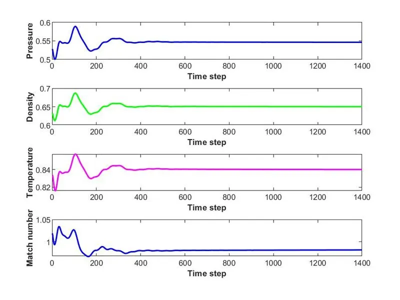
Fig(6) - For a conservative form of governing equation the plot between time step and primitive variables
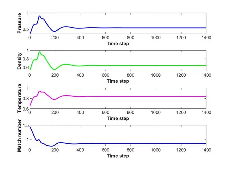
Fig(5) - For a non-conservative form of governing equation the plot between nozzle length and primitive variables
2nd Observation
Fig(2) - For a conservative form of governing equation the plot between nozzle length and primitive variables
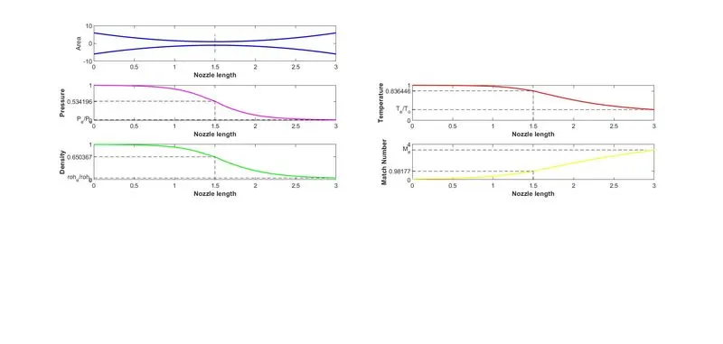
Fig(1) - For a non-conservative form of governing equation the plot between nozzle length and primitive variables
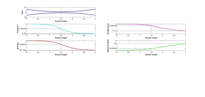
3rd Observation
Fig(4) - Comparision beween mass flow rate in different time step for conservative form of governing equation
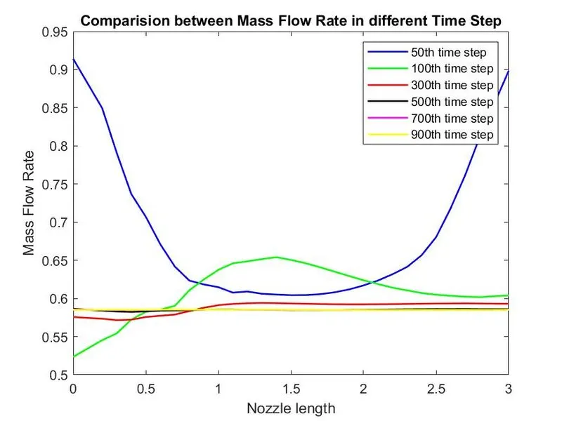
Fig(3) - Comparision beween mass flow rate in different time step for non-conservative form of governing equation
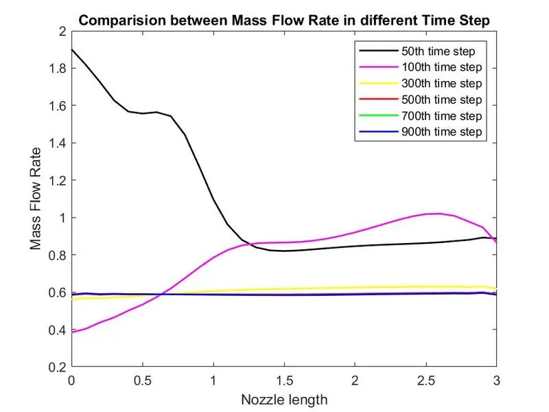
4th Observation
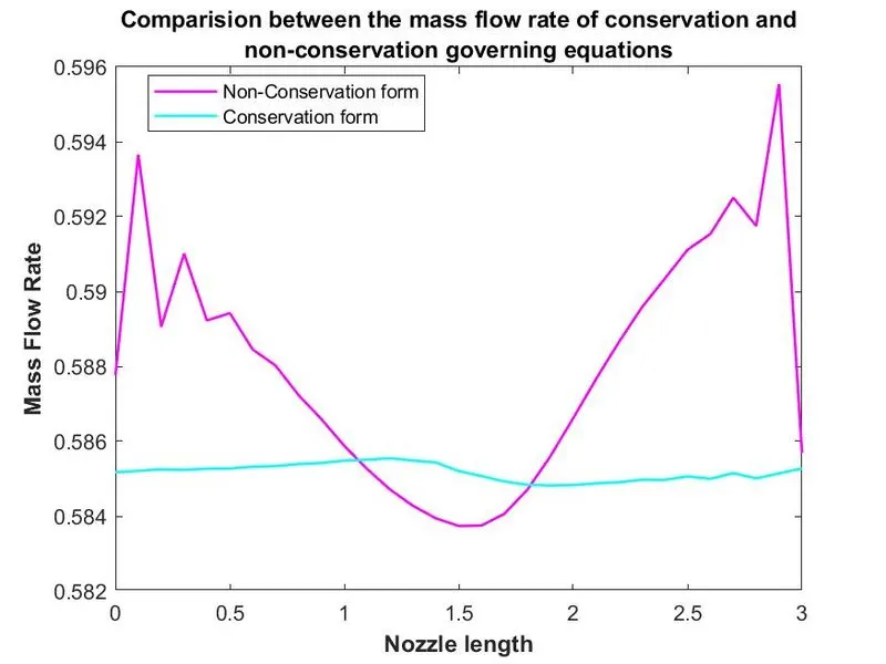
Fig(7) - Comparision beween mass flow rate in different nozzle length for non-conservative form and conservation form of governing equation in the basis of nozzle length
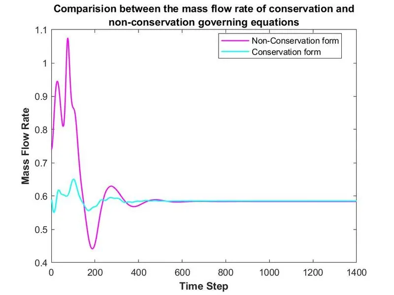
Fig(8) - Comparision beween mass flow rate in different time step for non-conservative form and conservative form of governing equation in the basis of time step
OBSERVATION:-
- We see that among figure(5) and figure(6) in Non-Conservation form the primitive variables are stabilized before the 400-time step but in the Conservation form the primitive variables are stabilized from 400-time step.
- We don't see any difference between figure(2) and figure(1). All the primitive variables are changing with nozzle length in the same manner.
- We observe that from figure(3) and figure(4) in starting the oscillation is higher but in figure(3) after nearly about 300-time steps the mass flow rate is stable but in figure(4) after 400-time steps the mass flow rate is stable.
- In the 4th observation, we see that the Non-Conservation form is very much oscillating in comparison to the Conservation form.
Grid Dependancy Test:-
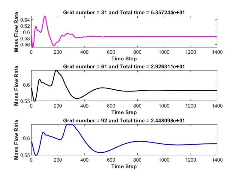
The grid dependancy test for Conservative form
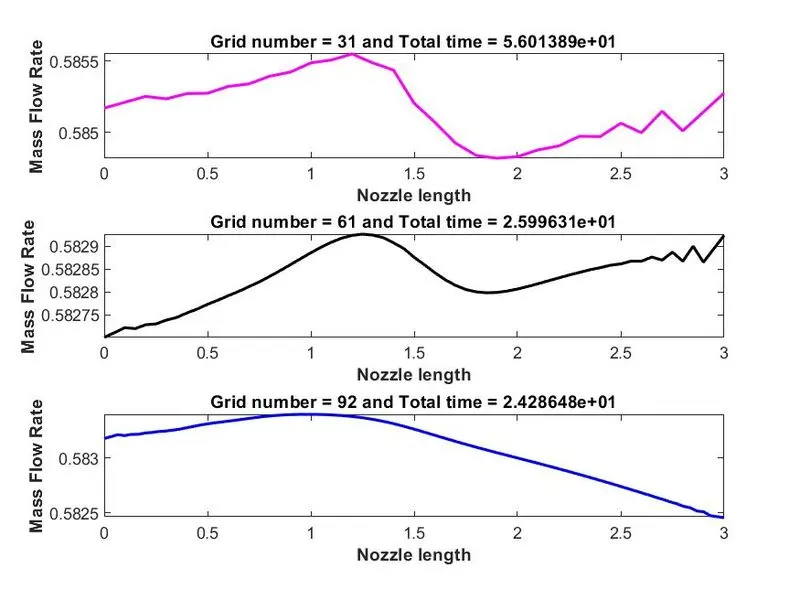
The grid dependancy test for Non-Conservative form
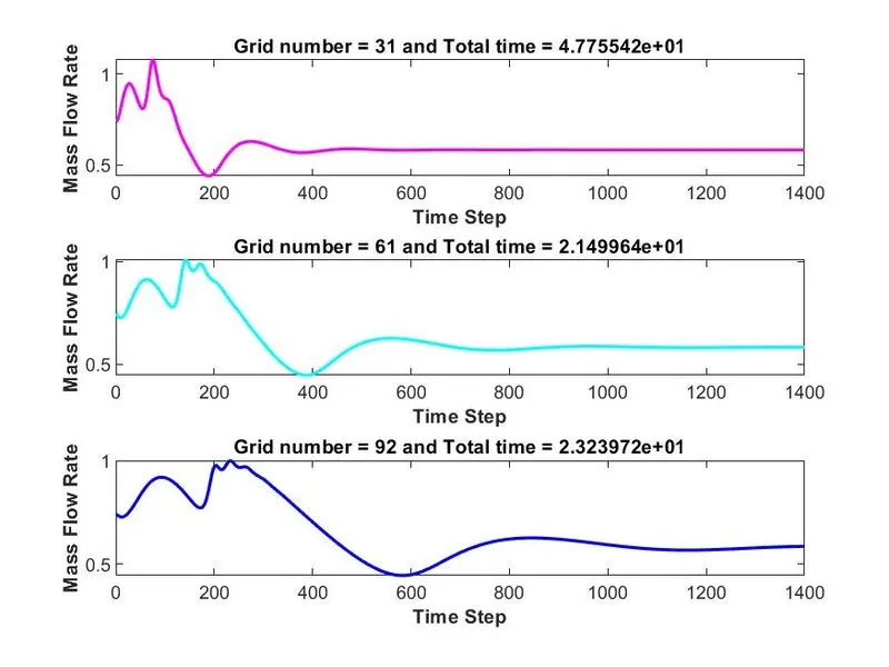
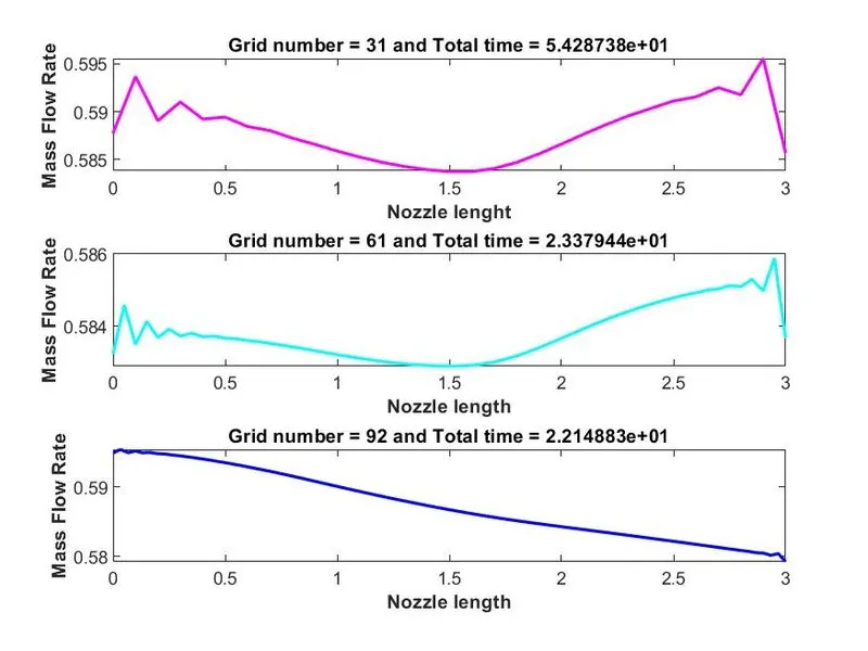
Observation of grid dependancy test:- From the figures, we see that with the increasing of grid number the total time is lesser and since the result is the same in all the cases but then only with the greater grid number the greater time step is taken to the stable. And also the throat value is different for conservative form and non-conservative form for higher grid numbers.
CONCLUSION:- So from the observation we can say that the primitive variables converge to a numerical steady-state faster when using the Non-Conservation form compared to the Conservation form. But in the case of the Non-Conservation form, the primitive variables like density, temperature, and velocity might experience a sudden jump across these discontinuities. When the governing equation is expressed using the primitive variables, there may develop large gradients in the solution to blow up. On the other hand, the flux variables possess an interesting property that they remain constant across shocks. So the Conservative form is more stable than the Non-Conservative form.
If we go to the conclusion of grid dependency test in all cases final result is the same but with the increasing of grid number we get the results sooner but when the grid number is 31 the throat value is the same for both the conservation and non-conservation form but for a higher value of grid number the throat value is different because we know Non-Conservative form is a more accurate comparison to the Conservative form. This is because the primitive variables are directly solved for in the governing equation of the Non-Conservative form.