Week 9 - FVM Literature Review

AIM:-Literature review on FVM and FDM and their differences also describe the needs for interpolation schemes and flux limiters in FVM by using the 1D linear heat conduction equation as an example.

THEORY:- Finite volume method (FVM) can be used on all differential equations, which can be written in the divergence form. This effectively writes the equation using divergence operators. The equation is then integrated over the volume. We can then apply Gauss’s theorem converting the volume integral over the divergence into a surface integral across the boundaries. The integral is therefore turned from integrating the differential of the dependent variable inside of the cells into surface integrals of the fluxes of the dependent variable across the boundary of the cells. These integrals can usually be calculated using suitable numerical approximation methods. This simplifies the differential equation substantially.

Finite volume method (FVM), like FEM, is based on an unstructured (e.g. triangular) mesh. Therefore, it is suitable for irregular and complex geometries. FVM has another advantage over FEM for fluid mechanic problems. So far, the numerical methods that we presented have been based on PDEs. By contrast, FVM is based on the integral form of the conservation laws, rather than their differential form.

The finite volume method (FVM) is a method for representing and evaluating partial differential equations in the form of algebraic equations. Similar to the finite difference method (FDM) or finite element method (FEM), values are calculated at discrete places on a meshed geometry.

Differences bewteen FVM and FDM

• A finite difference method (FDM) discretezation is based upon the differential form of the PDE to be solved. Each derivative is replaced with an approximate difference formula that can generallly be derived from a Taylor series expansion. The computational Domain is usually divided into grids and the solution will be obtained at each nodal point.
• A Finite volume method (FVM) discretezation is based upon the integral form of PDE to be solved (eg. conservation of mass, momentum or energy). The PDE is written in a form that can be solved for a given finite volume for cells. The coputational domain is discretized into finite volumes and then for every volume, the governing equations are solved. The resulting system of the equation usually involves fluxes of the conserved variables, and thus the calculation of fluxes is very important in FVM.
• The basic advantage of this method FVM is it doesnot require the use of structured grids, and the effort to convert the given mesh into a structured numerical grid internally is completely avoided.

• The approximations of surface and volume integrals require values of variable at location other than computational nodes of the CV
• values are obtained at these nodes by interpolation formula

Various interpolation methods are :-

1. Upwind interpolation
2. Linear interpolation
3. Quadratic upwind interpolation
4. Hybrid and TVD (Total varration Dimension) interpolation

1. Upwind interpolation

• This is the simplest numerical scheme thats why it is used earlier in the discretezation example.
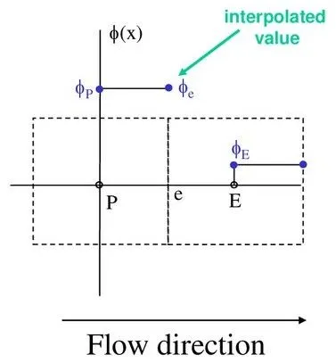
• We assume that the value of at the face is the same as the cell centered value in the cell upstream of the face.
• The main advantages are that it is easy to implement and that it results in very stable calculations, but it also very diffusive. Gradients in the flow field tend to be smeared out, as we will show later.

We would require upwind interpolation scheme which is essentially used for convection dominated problem, here the velocity at a given point direction of that whcich determinants the variable values to be used in the interpolation process, name upwind refers to the upstreams of the flow

The upwind interpolation for approximating the value of variable 'f' at the east face of the control volumeis given below

2. Linear interpolation

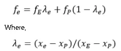
linear interpolation is a method of curve fitting using linear polynomials to construct new data points within the range of a discrete set of known data points.WE can approximate the value at the CV face center by linear interpolation of the values atthe two nearest computational nodes.

The linear interpolation is equivalent to the use of the central difference formula of the first order derivative, and hence, this scheme is also termed as central difference schem (CDS).This scheme is second order accurate and may produce oscillatory solutions.

Finite volume method for 1D steady state diffusion

Consider the steady state diffusion of a property in 1 domensional domain define in figure given below. The process is governed by this equation.

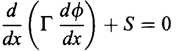
where is diffusion coeffient and S is the source term. Boundary values of at points A and B are prescribed.

Step 1 : Grid generation

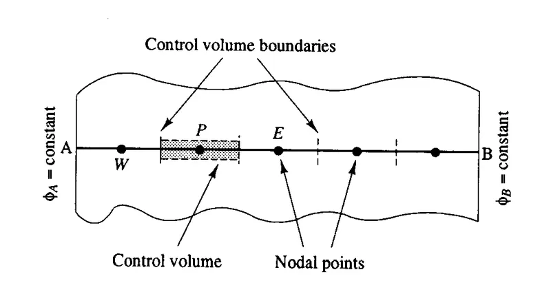
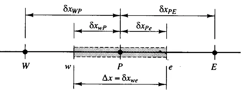
First step of FVM is to divide the domain into discreate control volumes. Let us place a number of nodal points in the space between A and B. The boundaries of control volumes are positined mid way between adjacent nodes. Thus each node is surrounded by a control volume or cell.

A general nodal point is identified by P and its neighbours in a one dimensional geometry, the nodes to the west to east, are W and E. The west side face of the control volume is 'w' and east side control volume is 'e'and dx = dxwe as defined in the figure below.

Step 2 : Discretezation

The key step of the FVM is the integration of the governing equation over a control volume to yield a discretised equation at its nodal point P. for the control volume defined above this gives us

here, A is the cross- sectional area of the control volume face, is the volume and is the average value of source S over the control volume. This above equation states that diffusive flux of leaving the east face minus the diffusive flux of entering the west face is equal to the generation of i.e, It constitues a balance equation for over the control volume.

In order to derive the useful forms of the descretized equations, the interface diffusion and the gradient 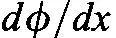at east and west are required. To caculate gradients at the control volume face of approximate distribution of properties between nodal points is used. Linear approximations seem very simplest way of calculating interface values and the gradients.

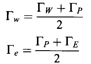and the diffusive flux terms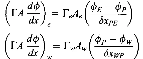

The source terms S may be the function of the dependent variable are

After substition of equations given above we got this equation as a final result.

Step 3 : Solution of equation

Discretised equation of the form above equation the final result must be set up at each of the nodal points in order to solve a problem.For control volumes that are adjacent tothe domain boundaries the general discretised equation is modified to incorporate boundary conditions.The resulting system of linear algebraic equations is then solved to obtain the distribution of the property at nodal points.

Flux limilters:-

Flux limiters are used in high resolution schemes – numerical schemes used to solve problems in science and engineering, particularly fluid dynamics, described by partial differential equations (PDE's). They are used in high resolution schemes, such as the MUSCL scheme, to avoid the spurious oscillations (wiggles) that would otherwise occur with high order spatial discretization schemes due to shocks, discontinuities or sharp changes in the solution domain. Use of flux limiters, together with an appropriate high resolution scheme, make the solutions total variation diminishing (TVD)

flux limiters are also referred to as slope limiters because they both have the same mathematical form, and both have the effect of limiting the solution gradient near shocks or discontinuities.

The main idea behind the construction of flux limiter schemes is to limit the spatial derivatives to realistic values – for scientific and engineering problems this usually means physically realisable and meaningful values. They are used in high resolution schemes for solving problems described by PDEs and only come into operation when sharp wave fronts are present. For smoothly changing waves, the flux limiters do not operate and the spatial derivatives can be represented by higher order approximations without introducing spurious oscillations. Consider the 1D semi-discrete scheme

and represent edge fluxes for the ith cell. If these edge fluxes can be represented by low and high resolution schemes, then a flux limiter can switch between these schemes depending upon the gradients close to the particular cell, as follows

,

,

where

low resolution flux,

high resolution flux,

flux limiter function,

r represents the ratio of successive gradients on the solution mesh, i.e.,

.

The limiter function is constrained to be greater than or equal to zero, i.e., . Therefore, when the limiter is equal to zero (sharp gradient, opposite slopes or zero gradient), the flux is represented by a low resolution scheme Similarly, when the limiter is equal to 1 (smooth solution), it is represented by a high resolution scheme