Week 9 - FVM Literature Review
Finite Volume Method (FVM )
The finite volume method (FVM) is a method for representing and evaluating partial differential equations in the form of algebraic equations. In the finite volume method, volume integrals in a partial differential equation that contain a divergence term are converted to surface integrals, using the divergence theorem. These terms are then evaluated as fluxes at the surfaces of each finite volume. Because the flux entering a given volume is identical to that leaving the adjacent volume, these methods are conservative. Another advantage of the finite volume method is that it is easily formulated to allow for unstructured meshes. The method is used in many cfd packages. "Finite volume" refers to the small volume surrounding each node point on a mesh. Since FVM based on unstructured mesh it is suitable for irregular and complex geometries.
Difference between FDM & FVM
| FINITE DIFFERENCE METHOD (FDM) | FINITE VOLUME METHOD (FVM) |
| Differential form of governing equations | Integral form of governing equations |
| Domain is discretized into finite discrete points | Domain is discretized into finite volumes |
| Defined on a regular/structured grid | Defined on any irregular/unstructured grid |
| Regular grids are suitable for very large scale simulations | Suitable for complex geometries |
| Solutions will be obtained on nodal points | Solutions will be obtained on centre of each cell |
| Depends on grid smoothness | Grid smoothness is not required since independent variables are integrated directly on the physical domain |
| Adaptive mesh refinement is not possible | Highly refined mesh can be obtained at the corners |
Solving steady state 1D heat conduction equation using FVM
Let 1D heat conduction equation is,
`del/(delx)(alpha(delT)/(delx))+S=0`
where, S = Source term
`alpha`=thermal diffusivity
Let's take a control volume 'P' and neighbouring volumes 'W' and 'E' as shown in below.
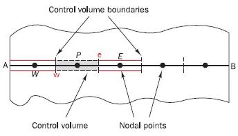
where, 'w' is the face between control volume(CV) 'W' and 'P'.
Similarly 'e' is the face between CV 'P' and 'E'.
Since it is FVM we need integral form of governing equation, So integrate the heat equation over the control volume 'P'.
`rArr``int_w^e (del/(delx)(alpha(delT)/(delx))+S)dV=0`
`rArr``int_w^e del/(delx)(alpha(delT)/(delx))dV+int_w^eSdV=0`
By simplifying,
`int_w^e del/(delx)(alpha(delT)/(delx))Adx+int_w^eSdV=0`
where dV=A*dx;
A = face area of the CV
dx = length of the CV
On further simplifying, we can write it as,
`[alphaA(delT)/(delx)]_w^e+barSdV=0`
where, `barS` is the average value of Source term.
`rArr``alphaA((delT)/(delx))_e-alphaA((delT)/(delx))_w+barSdV=0`
By using the 1st order approximation we have the FVM conservation equation like this,
`ubrace(ubrace(alphaA[(T_E-T_P)/(dx)])_("heat flux")-ubrace(alphaA[(T_P-T_W)/(dx)])_("heat flux"))_("flux terms")+barSdV=0`
Basically it says that,
heat flux out-heat flux in+source term=0
i.e, the amount of heat removed from a particular CV is conserved.
- Inorder to find out the temperature gradient terms we seek help from the neighbouring points. This is known as 'Gradient form'.
The need of Interpolation schemes in FVM
We know that, thermal diffusivity (`alpha`) is a function of temperature. If we need to estimate the value of `alpha` of any of these faces (east or west) we need to find out the temperature in the particular face. This means we need some kind of calculations to determine the temperature at particular faces. This is known as the 'Interpolation Scheme'. That's why we need interpolation schemes in FVM.
The interpolation scheme used in FVM are,
- Central Differencing Scheme
- Upwind Differencing Scheme
- Hybrid Differencing Scheme
- Power-Law Scheme
- Quadratic Upwind Differencing Scheme( QUICK scheme )
- Total variation and TVD schemes
The need of Flux Limiters in FVM
Most of us might have seen the behaviour of numerical schemes in order to capture shocks and discontinuity that arises in hyperbolic equations. Physically, these equations model the convective fluid flow. It has been observed that low-order schemes are usually stable but quite dissipative in nature around the points of discontinuity/shocks. On the other hand higher-order numerical schemes are unstable in nature and show oscillations in the vicinity of discontinuity.
The objective is to have highly accurate and stable oscillation free schemes. This kind of schemes are known as high resolution schemes. In 1984 Harten proposed the constuction and gave TVD criteria for such scheme. Here we talk only about using flux limiters function to construct high resolution schemes. The idea is to tune the numerical flux of high order and low order scheme using the flux limiter function in such a way that the resulting scheme gives a high order accuracy in the smooth region of flow and sticks with first order of accuracy in the vicinity of discontinuities.
Generally we can say that, the flux limiters are used in high resolution schemes to avoid oscillations that would occur with high order schemes due to shocks or discontinuities in the domain. They are used for limiting the spatial derivatives to realistic values.
Simply we can say that when we calculating gradients, we need to have those values bounded. Suppose if we have a shock flow problem then there will be a huge discontinuity. And when we calculate the gradients, it can be huge values. This should not happen. And because of that we need 'Flux Limiter'.