Week 3.5 - Deriving 4th order approximation of a 2nd order derivative using Taylor Table method

DERIVATION OF FOURTH ORDER APPROXIMATION OF SECOND ORDER DERIVATIVE BY DIFFERENT METHODS

• CENTRAL DIFFERENCE

To know about the number of nodes that we have to taken, we use the following expression.

For Central Schemes,

Number of nodes in stencil (N) = The order of accuracy (p) + The Order of derivative (q)-1

For Skewed Schemes,

Number of nodes in stencil (N) = The order of accuracy (p) + The Order of derivative (q)

Here we have Cental Difference Scheme,

So, N = p+q-1

N = 4+2-1

`:.` N = 5

Let,

`f''(x) = (a.f(i-2)+b.f(i-1)+c.f(i)+d.f(i+1)+e.f(i+2))/(Delta x^2)`

By Taylor series expansion,

`a.f(i-2) = a[ f(i)-(2Deltax)f'(i)+((2Deltax)^2f''(i))/(2!)-((2Deltax)^3f'''(i))/(3!)+((2Deltax)^4f''''(i))/(4!)-((2Deltax)^5f'''''(i))/(5!)]`

`b.f(i-1) = b[ f(i)-(Deltax)f'(i)+((Deltax)^2f''(i))/(2!)-((Deltax)^3f'''(i))/(3!)+((Deltax)^4f''''(i))/(4!)-((Deltax)^5f'''''(i))/(5!)]`

`c.f(i) = c.f(i)`

`d.f(i+1) = d[ f(i)+(Deltax)f'(i)+((Deltax)^2f''(i))/(2!)+((Deltax)^3f'''(i))/(3!)+((Deltax)^4f''''(i))/(4!)+((Deltax)^5f'''''(i))/(5!)]`

`e.f(i+2) = e[ f(i)+(2Deltax)f'(i)+((2Deltax)^2f''(i))/(2!)+((2Deltax)^3f'''(i))/(3!)+((2Deltax)^4f''''(i))/(4!)+((2Deltax)^5f'''''(i))/(5!)]`

Taylor's table,

	f(i)	`Deltaxf'(i)`	`Deltax^2f''(i)`	`Deltax^3f'''(i)`	`Deltax^4f''''(i)`	`Deltax^5f'''''(i)`
a.f(i-2)	a	-2a	2a	`-8/6a`	`16/24a`	`-32/120a`
b.f(i-1)	b	-b	`b/2`	`-b/6`	`b/24`	`-b/120`
c.f(i)	c	0	0	0	0	0
d.f(i+1)	d	d	`d/2`	`d/6`	`d/24`	`d/120`
e.f(i+2)	e	2e	2e	`8/6e`	`16/24e`	`32/120e`
`sum`	0	0	1	0	0	0

We have 6 equations and 5 unknowns.

So,

`a+b+c+d+e=0`........(1)

`-2a-b+d+2e=0`........(2)

`2a+b/2+d/2+2e=1`........(3)

`-8/6a-b/6+d/6+8/6e=0`........(4)

`16/24a+b/24+d/24+16/24e=0`........(5)

In matrix form,

`[[1,1,1,1,1],[-2,-1,0,1,2],[2,1/2,0,1/2,2],[-8/6,-1/6,0,1/6,8/6],[16/24,1/24,0,1/24,16/24]]xx[[a],[b],[c],[d],[e]] = [[0],[0],[1],[0],[0]]`

On further solving we get the values of the unknowns,

i.e,

a = -0.0833

b = 1.3333

c = -2.5

d = 1.3333

e = -0.0833

Therefore

`f''(x) = (-0.0833f(i-2)+1.3333f(i-1)-2.5f(i)+1.3333f(i+1)-0.0833f(i+2))/(Delta x^2)`

• SKEWED RIGHT SIDED DIFFERENCE

Number of nodes in the stencil, N = p+q

N = 4+2

`:.` N = 6

Let,

`f''(x) = (a.f(i)+b.f(i+1)+c.f(i+2)+d.f(i+3)+e.f(i+4)+g.f(i+5))/(Delta x^2)`

By Taylor series expansion,

`a.f(i) = a.f(i)`

`b.f(i+1) = b[ f(i)+(Deltax)f'(i)+((Deltax)^2f''(i))/(2!)+((Deltax)^3f'''(i))/(3!)+((Deltax)^4f''''(i))/(4!)+((Deltax)^5f'''''(i))/(5!)]`

`c.f(i+2) = c[ f(i)+(2Deltax)f'(i)+((2Deltax)^2f''(i))/(2!)+((2Deltax)^3f'''(i))/(3!)+((2Deltax)^4f''''(i))/(4!)+((2Deltax)^5f'''''(i))/(5!)]`

`d.f(i+3) = d[ f(i)+(3Deltax)f'(i)+((3Deltax)^2f''(i))/(2!)+((3Deltax)^3f'''(i))/(3!)+((3Deltax)^4f''''(i))/(4!)+((3Deltax)^5f'''''(i))/(5!)]`

`e.f(i+4) = e[ f(i)+(4Deltax)f'(i)+((4Deltax)^2f''(i))/(2!)+((4Deltax)^3f'''(i))/(3!)+((4Deltax)^4f''''(i))/(4!)+((4Deltax)^5f'''''(i))/(5!)]`

`g.f(i+5) = g[ f(i)+(5Deltax)f'(i)+((5Deltax)^2f''(i))/(2!)+((5Deltax)^3f'''(i))/(3!)+((5Deltax)^4f''''(i))/(4!)+((5Deltax)^5f'''''(i))/(5!)]`

Taylor's table,

	f(i)	`Deltaxf'(i)`	`Deltax^2f''(i)`	`Deltax^3f'''(i)`	`Deltax^4f''''(i)`	`Deltax^5f'''''(i)`
a.f(i)	a	0	0	0	0	0
b.f(i+1)	b	b	`b/2`	`b/6`	`b/24`	`b/120`
c.f(i+2)	c	2c	2c	`8/6c`	`16/24c`	`32/120c`
d.f(i+3)	d	3d	`9/2d`	`27/6d`	`81/24d`	`243/120d`
e.f(i+4)	e	4e	8e	`64/6e`	`256/24e`	`1024/120e`
g.f(i+5)	g	5g	`25/2g`	`125/6g`	`625/24g`	`3125/120g`
`sum`	0	0	1	0	0	0

We have 6 equations and 6 unknowns.

So,

`a+b+c+d+e+g=0`........(1)

`b+2c+3d+4e+5g = 0`........(2)

`b/2+2c+9/2d+8e+25/2g = 1`........(3)

`b/6+8/6c+27/6d+64/6e+125/6g = 0`........(4)

`b/24+16/24c+81/24d+256/24e+625/24g = 0`........(5)

`b/120+32/120c+243/120d+1024/120e+3125/120g = 0`........(6)

In matrix form,

`[[1,1,1,1,1,1],[0,1,2,3,4,5],[0,1/2,2,9/2,8,25/2],[0,1/6,8/6,27/6,64/6,125/6],[0,1/24,16/24,81/24,256/24,625/24],[0,1/120,32/120,243/120,1024/120,3125/120]]xx[[a],[b],[c],[d],[e],[g]] = [[0],[0],[1],[0],[0],[0]]`

On further solving we get the values of the unknowns,

i.e,

a = 3.7500

b = -12.8333

c = 17.8333

d = -13.0000

e = 5.0833

g = -0.8333

Therefore

`f''(x) = (3.7500f(i)-12.8333f(i+1)+17.8333f(i+2)-13.0000f(i+3)+5.0833f(i+4)-0.8333f(i+5))/(Delta x^2)`

• SKEWED LEFT SIDED DIFFERENCE

Number of nodes in the stencil, N = p+q

N = 4+2

`:.` N = 6

Let,

`f''(x) = (a.f(i-5)+b.f(i-4)+c.f(i-3)+d.f(i-2)+e.f(i-1)+g.f(i))/(Delta x^2)`

By Taylor series expansion,

`a.f(i-5) = a[ f(i)-(5Deltax)f'(i)+((5Deltax)^2f''(i))/(2!)-((5Deltax)^3f'''(i))/(3!)+((5Deltax)^4f''''(i))/(4!)-((5Deltax)^5f'''''(i))/(5!)]`

`b.f(i-4) = b[ f(i)-(4Deltax)f'(i)+((4Deltax)^2f''(i))/(2!)-((4Deltax)^3f'''(i))/(3!)+((4Deltax)^4f''''(i))/(4!)-((4Deltax)^5f'''''(i))/(5!)]`

`c.f(i-3) = c[ f(i)-(3Deltax)f'(i)+((3Deltax)^2f''(i))/(2!)-((3Deltax)^3f'''(i))/(3!)+((3Deltax)^4f''''(i))/(4!)-((3Deltax)^5f'''''(i))/(5!)]`

`d.f(i-2) = d[ f(i)-(2Deltax)f'(i)+((2Deltax)^2f''(i))/(2!)-((2Deltax)^3f'''(i))/(3!)+((2Deltax)^4f''''(i))/(4!)-((2Deltax)^5f'''''(i))/(5!)]`

`e.f(i-1) = e[ f(i)-(Deltax)f'(i)+((Deltax)^2f''(i))/(2!)-((Deltax)^3f'''(i))/(3!)+((Deltax)^4f''''(i))/(4!)-((Deltax)^5f'''''(i))/(5!)]`

`g.f(i) = g.f(i)`

Taylor's table,

	f(i)	`Deltaxf'(i)`	`Deltax^2f''(i)`	`Deltax^3f'''(i)`	`Deltax^4f''''(i)`	`Deltax^5f'''''(i)`
a.f(i-5)	a	-5a	`25/2a`	`-125/6a`	`625/24a`	`-3125/120a`
b.f(i-4)	b	-4b	8b	`-64/6b`	`256/24b`	`-1024/120b`
c.f(i-3)	c	-3c	`9/2c`	`-27/6c`	`81/24c`	`-243/120c`
d.f(i-2)	d	-2d	2d	`-8/6d`	`16/24d`	`-32/120d`
e.f(i-1)	e	-e	`e/2`	`-e/6`	`e/24`	`-e/120`
g.f(i)	g	0	0	0	0	0
`sum`	0	0	1	0	0	0

We have 6 equations and 6 unknowns.

So,

`a+b+c+d+e+g=0`........(1)

`-5a-4b-3c-2d-e = 0`........(2)

`25/2a+8b+9/2c+2d+e/2 = 1`........(3)

`-125/6a-64/6b-27/6c-8/6d-e/6 = 0`........(4)

`625/24a+256/24b+81/24c+16/24d+e/24 = 0`........(5)

`-3125/120a-1024/120b-243/120c-32/120d-e/120 = 0`........(6)

In matrix form,

`[[1,1,1,1,1,1],[-5,-4,-3,-2,-1,0],[25/2,8,9/2,2,1/2,0],[-125/6,-64/6,-27/6,-8/6,-1/6,0],[625/24,256/24,81/24,16/24,1/24,0],[-3125/120,-1024/120,-243/120,-32/120,-1/120,0]]xx[[a],[b],[c],[d],[e],[g]] = [[0],[0],[1],[0],[0],[0]]`

On further solving we get the values of the unknowns,

i.e,

a = -0.8333

b = 5.0833

c = -13.0000

d = 17.8333

e = -12.8333

g = 3.7500

Therefore

`f''(x) = (-0.8333f(i-5)+5.0833f(i-4)-13.0000f(i-3)+17.8333f(i-2)-12.8333f(i-1)+3.7500f(i))/(Delta x^2)`

EXPLANATION

The matrix is solved by by using the following steps,

`[A][X] = [B]`

then,

`[X] = [A]^-1[B]`

It is solved by using MATLAB.

For finding `[A]^-1`, we use 'inverse' command in MATLAB.

i.e, the command for finding `[X]` is,

X = inv(A)*B;

FUNCTION CODE FOR 4TH ORDER CENTRAL DIFFERENCE SCHEME

function fourth_order_central_difference_error = fourth_order_central_difference_approx(x,dx);


%f(x) = exp(x)*cos(x)

%Analytical derivative
analytical_derivative = -2*exp(x)*sin(x);

%numerical derivative
fourth_order_central_difference = ((-0.0833333333333333*exp(x-2*dx)*cos(x-2*dx))+(1.3333333333333333*exp(x-dx)*cos(x-dx))-(2.5*exp(x)*cos(x))+(1.3333333333333333*exp(x+dx)*cos(x+dx))-(0.0833333333333333*exp(x+2*dx)*cos(x+2*dx)))/(dx^2);

%error
fourth_order_central_difference_error = abs(fourth_order_central_difference - analytical_derivative);

end

FUNCTION CODE FOR 4TH ORDER SKEWED RIGHT SIDED DIFFERENCE

function fourth_order_skewed_right_error = fourth_order_skewed_right_difference_approx(x,dx);


%f(x) = exp(x)*cos(x)

%Analytical derivative
analytical_derivative = -2*exp(x)*sin(x);

%numerical derivative
fourth_order_skewed_right_difference = ((3.75*exp(x)*cos(x))-(12.8333333333333333*exp(x+dx)*cos(x+dx))+(17.8333333333333333*exp(x+2*dx)*cos(x+2*dx))-(13*exp(x+3*dx)*cos(x+3*dx))+(5.0833333333333333*exp(x+4*dx)*cos(x+4*dx))-(0.8333333333333333*exp(x+5*dx)*cos(x+5*dx)))/(dx^2);
%error
fourth_order_skewed_right_error = abs(fourth_order_skewed_right_difference - analytical_derivative);

end

FUNCTION CODE FOR 4TH ORDER SKEWED LEFT SIDED DIFFERENCE

function fourth_order_skewed_left_error = fourth_order_skewed_left_difference_approx(x,dx);


%f(x) = exp(x)*cos(x)

%Analytical derivative
analytical_derivative = -2*exp(x)*sin(x);

%numerical derivative
fourth_order_skewed_left_difference = ((-0.8333333333333333*exp(x-5*dx)*cos(x-5*dx))+(5.0833333333333333*exp(x-4*dx)*cos(x-4*dx))-(13.0000*exp(x-3*dx)*cos(x-3*dx))+(17.8333333333333333*exp(x-2*dx)*cos(x-2*dx))-(12.8333333333333333*exp(x-dx)*cos(x-dx))+(3.7500*exp(x)*cos(x)))/(dx^2);
%error
fourth_order_skewed_left_error = abs(fourth_order_skewed_left_difference - analytical_derivative);

end

MAIN PROGRAM CODE

clear all
close all
clc

%Main program

%analytical function
%f(x) = exp(x)*cos(x)

%given values

x = pi/3;
dx = linspace(pi/400,pi/4,200);

%loop

for i = 1:length(dx)
    
    error_cds(i) = fourth_order_central_difference_approx(x,dx(i));
    error_skewed_right(i) = fourth_order_skewed_right_difference_approx(x,dx(i));
    error_skewed_left(i) = fourth_order_skewed_left_difference_approx(x,dx(i));
    
end

%plotting

loglog(dx,error_cds,'g','linewidth',1.5)
hold on
loglog(dx,error_skewed_right,'b','linewidth',1.5)
hold on
loglog(dx,error_skewed_left,'r','linewidth',1.5)
legend('central difference fourth order','skewed right fourth order','skewed left fourth order','location','best')
xlabel('dx')
ylabel('error')
title('dx vs Error')

RESULT

• GRAPH

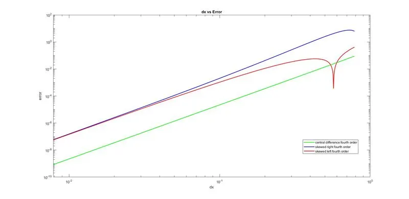
• why a skewed scheme is useful? What can a skewed scheme do that a CD scheme cannot?

When there are no nodes at the boundaries we can't able to use Central difference scheme. Because in CDS it needs the nodes from both sides. Such cases Skewed schemes are useful to approximate. Because Skewed schemes are need the nodes in one direction.