Week 7 - Simulation of a 1D Super-sonic nozzle flow simulation using Macormack Method
In this problem we consider the steady, isentropic flow through a convergent divergent nozzle as shown below.
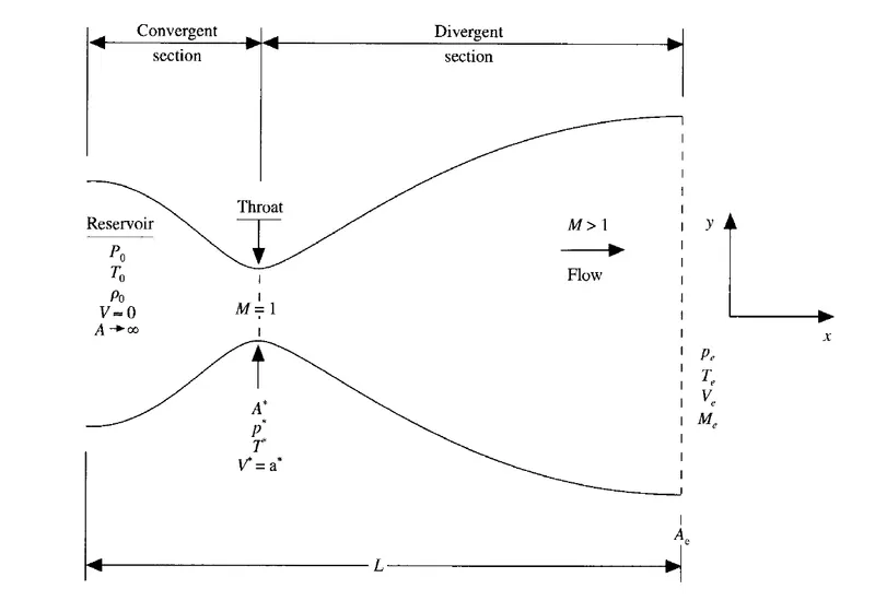
The flow at the inlet to the nozzle comes from a reservoir where the pressure and temperature are denoted by `p_0 and T_0` respectively. The cross-sectional area of the reservoir is large(`Ararroo`), and hence the velocity is very small(`Vrarr0`). Thus `p_0 and T_0` are stagnation values. The flow expands isentropically to supersonic speeds at the nozzle exit, where the exit pressure,temperature,velocity and Mach number are denoted by `p_e,T_e,V_e and M_e` respectively. The flow is locally subsonic in the convergent section of the nozzle, sonic at the throat and supersonic at the divergent section. The sonic flow(M=1) at the throat means that the local velocity at this location is equal to the local speed of sound. So at throat velocity is `V=V^**=a^**`. Similarly the area, pressure and temperature are deonted by `A^**,p^** and T^**`.
We assume that at a given section, where the cross-sectional area is `A`, the flow properties are uniform across the section. Hence although the area of the nozzle changes as a function of distance along the nozzle `x`, therefore in reality the flow field is two-dimensional, we make assumption that the flow properties vary along with `x`; this is tantamount to assuming uniform flow properties across any given cross-section. Such flow is defined as 'Quasi one dimensional flow'.
Then we have to find out the Governing equation for this problem(both Non-conservative and Conservative form). Here we employing the Non-dimensional forms of governing equations.
So we need to Non-dimensionalize the variables also.
Non-dimensional temperature, `T'=T/T_0`
Non-dimensional density, `rho'=rho/rho_0`
Non-dimensional length, `x'=x/L`
where L is the length of the nozzle
Non-dimensional velocity, `V'=V/a_0`
where `a_0` is the speed of the sound in the reservoir. `a_0=sqrt(gammaRT)`
Non-dimensional time, `t'=t/(L/a_0)`
Non-dimensional area, `A'=A/A^**`
Mach number, `M=V/a`
In terms of non dimensional velocity and temperature, this equation can be rewritten as
`M=(V')/sqrt(T)`
After finding out the Governing equations for both terms, the next step is solving by Macormack method.
Macormack Method
In the normal case solving is done by with an initial condition and move onto the next time step with help of suitable discretization scheme. In Macormack Method we are not going directly into the next time step. Before going to the next time step we have to do the predictor step and corrector step. Macormack Method consist of mainly 5 steps.
- Predictor step
- Intermediate solution update
- Corrector step
- Averaging time derivative
- Final solution update
example
Let 'f' be any function, and we are solving using Macormack method.
- Predictor step
Here we have to find out the time derivative. In this step we employ forward difference scheme for the spacial terms.
`((delf)/(delt))_p`
- Intermediate solution update
`f^**=f_i+((delf)/(delt))_pdt`
- Corrector step
Like the predictor step, here we need to find out the time derivative. But here we employing backward difference scheme for spacial terms. Also we have to use the updated values obtained from the predictor step(`f^**`) here.
`((delf^**)/(delt))_c`
- Averaging
Here we averaging the results obtained from the predictor step and corrector step
`((delf)/(delt))_(avg)=[((delf)/(delt))_p+((delf^**)/(delt))_c]/2`
- Final solution update
`f=f_i+((delf)/(delt))_(avg)dt`
NON DIMENSIONAL GOVERNING EQUATIONS SOLVING
Area profile
`A=1+2.2(x-1.5)^2`
let `0<=x<=3`
Calculation of time step
`dt=C.dx/(V+a)`
where C is the CFL number
V is the local velocity
a is the speed of sound
Mass flow rate calculation
Mass flow rate = `rhoAV`
- NON-CONSERVATIVE FORM
Continuity equation
`(del(rho'A'))/(delt')=-rho'(delV')/(delx')-rho'V'(del(lnA))/(delx')-V'(delrho')/(delx')`
Momentum equation
`(delV')/(delt')=-V'(delV')/(delx')-1/gamma((delT')/(delx')+(T')/(rho')(delrho')/(delx'))`
Energy equation
`(delT')/(delt')=-V'(delT')/(delx')-(gamma-1)T'[(delV')/(delx')+V'(del(lnA))/(delx')]`
Initial conditions are,
`rho'=1-0.3146x'`
`T'=1-0.2314x'`
`V'=(0.1+1.09x')T'^(1/2)`
By Marcomack method,
Predictor step,



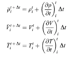
Intermediate solution update,
Corrector step,
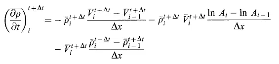

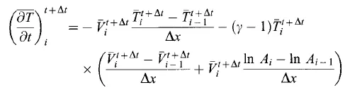
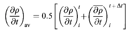
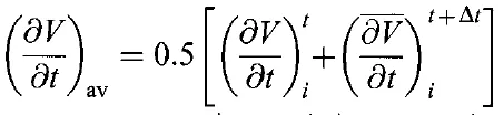
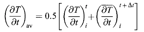
Averaging time derivatives,
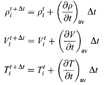
Final solution update,
Boundary conditions
Subsonic inflow boundary,
`V_1=2V_2-V_3`
Subsonic outflow boundary,
`V_n=2V_(n-1)-V_(n-2)`
`rho_n=2rho_(n-1)-rho_(n-2)`
`T_n=2T_(n-1)-T_(n-2)`
- CONSERVATIVE FORM
Continuity equation
`(del(rho'A'))/(delt')+(del(rho'A'V'))/(delx')=0`
Momentum equation
`(del(rho'A'V'))/(delt')+(del[rho'A'V'^2+(1/gamma)p'A'])/(delx')=1/gammap'(delA')/(delx')`
Energy equation
`(del[rho'((e')/(gamma-1)+gamma/2V'^2)A'])/(delt')+(del[rho'((e')/(gamma-1)+gamma/2V'^2)V'A'+p'A'V'])/(delx')=0`
To simplify these equations we introduce some new terms which include the solution vector `U`, Flux vector `F` and source term `J`.
`U_1=rho'A'`
`U_2=rho'A'V'`
`U_3=rho'((e')/(gamma-1)+gamma/2V'^2)A'`
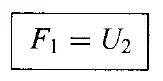
`F_1=rho'A'V'`
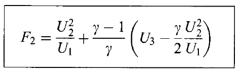
`F_2=rho'A'V'^2+(1/gamma)p'A'`
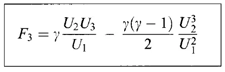
`F_3=rho'((e')/(gamma-1)+gamma/2V'^2)V'A'+p'A'V'`
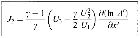
`J_2=1/gammap'(delA')/(delx')`
By using these terms we can rewrite the equations as follows,
`(delU_1)/(delt')=-(delF_1)/(delx')`
`(delU_2)/(delt')=-(delF_2)/(delx')+J_2`
`(delU_3)/(delt')=-(delF_3)/(delx')`
The primitive variables can be calculated as follows,
`rho'=U_1/(A')`
`V'=U_2/U_1`
`T'=e'=(gamma-1)(U_3/U_1-gamma/2V'^2)`
`p'=rho'T'`
Expressing flex terms and source terms in terms of solution vectors,
Initial conditions are,
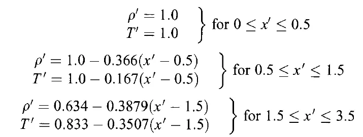
solution variable initialization,
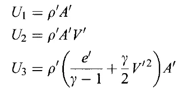
By Macormack method,
The predictor step,
`((delU_1)/(delx))_i^t=-((F_(1(i+1))^t-F_(1(i))^t)/dx)`
`((delU_2)/(delx))_i^t=-((F_(2(i+1))^t-F_(2(i))^t)/dx)+ubrace([(1/gamma)rho_iT_i((A_(i+1)-A_(i))/dx)])_("J_2")`
`((delU_3)/(delx))_i^t=-((F_(3(i+1))^t-F_(3(i))^t)/dx)`
Intermediate solution update,
`(bar U_1)_i^(t+dt)=(U_1)_i^t+((delU_1)/(delt))_i^tdt`
`(bar U_2)_i^(t+dt)=(U_2)_i^t+((delU_2)/(delt))_i^tdt`
`(bar U_3)_i^(t+dt)=(U_3)_i^t+((delU_3)/(delt))_i^tdt`
Then update the primitive variables.
The corrector step,
`((del barU_1)/(delx))_i^t=-((bar F_(1(i))^t-bar F_(1(i-1))^t)/dx)`
`((delbar U_2)/(delx))_i^t=-((bar F_(2(i))^t-bar F_(2(i-1))^t)/dx)+ubrace([(1/gamma)rho_iT_i((A_(i)-A_(i-1))/dx)])_("J_2")`
`((del barU_3)/(delx))_i^t=-((bar F_(3(i))^t-bar F_(3(i-1))^t)/dx)`
Averaging,
`((delU_1)/(delt))_(avg)=[((delU_1)/(delt))_i^t+((delbar U_1)/(delt))_i^t]/2`
`((delU_2)/(delt))_(avg)=[((delU_2)/(delt))_i^t+((delbar U_2)/(delt))_i^t]/2`
`((delU_3)/(delt))_(avg)=[((delU_3)/(delt))_i^t+((delbar U_3)/(delt))_i^t]/2`
Final solution update,
`(U_1)_i^(t+dt)=(U_1)_i^t+((delU_1)/(delt))_(avg)dt`
`(U_2)_i^(t+dt)=(U_2)_i^t+((delU_2)/(delt))_(avg)dt`
`(U_3)_i^(t+dt)=(U_3)_i^t+((delU_3)/(delt))_(avg)dt`
After this step we need to update the primitive variables.
Boundary conditions
Subsonic inflow boundary,
`U_(1(i=1))=(rho'A')_(i=1)=A'_(i=1)=`Fixed value
`U_(2(i=1))=2U_(2(i=2))-U_(2(i=3))`
`U_3=U_1(T_1/(gamma-1)+gamma/2V'^2)`
Supersonic outflow boundary,
`(U_1)_n=2(U_1)_(n-1)-(U_1)_(n-2)`
`(U_2)_n=2(U_2)_(n-1)-(U_2)_(n-2)`
`(U_3)_n=2(U_3)_(n-1)-(U_3)_(n-2)`
MATLAB PROGRAM
- Main Program Code
% main function supersonic flow

clear all
close all
clc

%inputs
n=31;
x=linspace(0,3,n);
dx=x(2)-x(1);
gamma = 1.4;
%area
a = 1+2.2*(x-1.5).^2;
%cfl number
cfl = 0.5;
%time step
nt = 1400;

%non conservative
[rho,v,t,p,m,mfr,m_nc,p_nc,rho_nc,t_nc] = non_conservative(x,cfl,dx,nt,n,gamma);

%conservative
[rho_c,v_c,t_c,p_c,m_c,mfr_c,m_c_t,p_c_t,rho_c_t,t_c_t] = conservative(x,cfl,dx,nt,n,gamma,a);


%plotting

% 1.primitive variables vs x
%non conservative form


figure(3)
%Mach number
subplot(4,1,1)
plot(x,m)
xlabel('x')
ylabel('Mach number')
title('Primitive variables vs x(non conservative)')
grid on


subplot(4,1,2)
plot(x,p)
xlabel('x')
ylabel('Pressure')
grid on

subplot(4,1,3)
plot(x,rho)
xlabel('x')
ylabel('Density')
grid on

subplot(4,1,4)
plot(x,t)
xlabel('x')
ylabel('Temperature')
grid on

%conservative form
figure(4)

subplot(4,1,1)
plot(x,m_c)
xlabel('x')
ylabel('Mach number')
title('Primitive variables vs x(conservative)')
grid on

subplot(4,1,2)
plot(x,p_c)
xlabel('x')
ylabel('Pressure')
grid on

subplot(4,1,3)
plot(x,rho_c)
xlabel('x')
ylabel('Density')
grid on

subplot(4,1,4)
plot(x,t_c)
xlabel('x')
ylabel('Temperature')
grid on


% 2.time wise variation of primitive variable

%mach number
figure(5)
plot(1:nt, m_nc)
hold on
plot(1:nt, m_c_t)
xlabel('time step')
ylabel('mach number')
legend('non conservative','conservative')
title('Time wise variation of Mach number')
grid on

%pressure
figure(6)
plot(1:nt, p_nc)
hold on
plot(1:nt, p_c_t)
xlabel('time step')
ylabel('pressure')
legend('non conservative','conservative')
title('Time wise variation of Pressure')
grid on

%density
figure(7)
plot(1:nt, rho_nc)
hold on
plot(1:nt, rho_c_t)
xlabel('time step')
ylabel('density')
legend('non conservative','conservative')
title('Time wise variation of Density')
grid on

%temperature
figure(8)
plot(1:nt, t_nc)
hold on
plot(1:nt, t_c_t)
xlabel('time step')
ylabel('temperature')
legend('non conservative','conservative')
title('Time wise variation of Temperature')
grid on


% 4.comparison of normalized mass flow rate distributions of both forms
figure(9)
plot(x,mfr,'linewidth',1.5)
hold on
plot(x,mfr_c,'linewidth',1.5)
xlabel('x')
ylabel('Mass flow distribution')
legend({'non conservative','conservative'},'location','best')
title('Mass flow rate distribution')
grid on- FUNCTION CODE for Non-Conservative form
function [rho,v,t,p,m,mfr,m_nc,p_nc,rho_nc,t_nc] = non_conservative(x,cfl,dx,nt,n,gamma,a)

    %initial profiles
    rho = 1-0.3146*x;           %density
    t = 1-0.2314*x;             %temperature
    v = (0.1+1.09*x).*t.^0.5;   %velocity

    %time step
    dt = min((cfl*dx)./(v+sqrt(t)));

    %outer time loop
    for k=1:nt

        rho_old = rho;
        t_old = t;
        v_old = v;

        %predictor method

        for j=2:n-1

            dvdx=(v(j+1)-v(j))/dx;
            drhodx=(rho(j+1)-rho(j))/dx;
            dtdx=(t(j+1)-t(j))/dx;
            dlogadx=(log(a(j+1))-log(a(j)))/dx;

            %continuity equation
            drhodt_p(j) = -rho(j)*dvdx-rho(j)*v(j)*dlogadx-v(j)*drhodx;

            %momentum equation
            dvdt_p(j) = -v(j)*dvdx-(1/gamma)*(dtdx+(t(j)/rho(j))*drhodx);

            %energy equation
            dtdt_p(j) = -v(j)*dtdx-(gamma-1)*t(j)*(dvdx+v(j)*dlogadx);

            %solution update
            rho(j) = rho(j)+drhodt_p(j)*dt;
            v(j) = v(j)+dvdt_p(j)*dt;
            t(j) = t(j)+dtdt_p(j)*dt;

        end


        %corrector method

        for j=2:n-1

            dvdx=(v(j)-v(j-1))/dx;
            drhodx=(rho(j)-rho(j-1))/dx;
            dtdx=(t(j)-t(j-1))/dx;
            dlogadx=(log(a(j))-log(a(j-1)))/dx;

            %continuity equation
            drhodt_c(j) = -rho(j)*dvdx-rho(j)*v(j)*dlogadx-v(j)*drhodx;

            %momentum equation
            dvdt_c(j) = -v(j)*dvdx-(1/gamma)*(dtdx+(t(j)/rho(j))*drhodx);

            %energy equation
            dtdt_c(j) = -v(j)*dtdx-(gamma-1)*t(j)*(dvdx+v(j)*dlogadx);

        end

        %computing average time derivative

        drhodt = 0.5*(drhodt_p+drhodt_c);
        dvdt = 0.5*(dvdt_p+dvdt_c);
        dtdt = 0.5*(dtdt_p+dtdt_c);

        %final solution update

        for i=2:n-1
            rho(i) = rho_old(i)+drhodt(i)*dt;
            v(i) = v_old(i)+dvdt(i)*dt;
            t(i) = t_old(i)+dtdt(i)*dt;
        end


        %applying boundary conditions

        %inlet
        v(1) = 2*v(2)-v(3);

        %outlet
        v(n) = 2*v(n-1)-v(n-2);
        rho(n) = 2*rho(n-1)-rho(n-2);
        t(n) = 2*t(n-1)-t(n-2);

        %Primitive variables updation
        p=rho.*t;       %pressure
        m=v./(t.^0.5);  %mach number
        mfr=rho.*a.*v;  %mass flow rate

        %Primitive variables at throat
        m_nc(k) = m(16);
        p_nc(k) = p(16);
        rho_nc(k) = rho(16);
        t_nc(k) = t(16);

        % plotting mass flow rate distribution inside nozzle at different time
        % steps
        figure(1)
        if k==50
            plot(x,mfr,'linewidth',1.5)
            hold on
        elseif k==100
            plot(x,mfr,'linewidth',1.5)
            hold on
        elseif k==150
            plot(x,mfr,'linewidth',1.5)
            hold on
        elseif k==300
            plot(x,mfr,'linewidth',1.5)
            hold on
        elseif k==600
            plot(x,mfr,'linewidth',1.5)
            hold on
        elseif k==900
            plot(x,mfr,'linewidth',1.5)
            hold on
        elseif k==1400
            plot(x,mfr,'linewidth',1.5)

        end


    end
    xlabel('x')
    ylabel('mass flow rate')
    legend('50 time steps','100 time steps','150 time steps','300 time steps','600 time steps','900 time steps','1400 time steps')
    title('mass flow distribution inside the nozzle at different time steps(non conservative method)')
    grid on

end- FUNCTION CODE for Conservative form
function [rho_c,v_c,t_c,p_c,m_c,mfr_c,m_c_t,p_c_t,rho_c_t,t_c_t] = conservative(x,cfl,dx,nt,n,gamma,a)

    %initial profiles
    for i=1:n

        if x(i)>=0 && x(i)<=0.5
            %Density
            rho_c(i) = 1.0;
            %temperature
            t_c(i) = 1.0;

        elseif x(i)>=0.5 && x(i)<=1.5

            rho_c(i) = 1 - (0.366*(x(i)-0.5));
            t_c(i) = 1 - (0.167*(x(i)-0.5));

        elseif x(i)>=1.5 && x(i)<=3.5

            rho_c(i) = 0.634 - (0.3879*(x(i)-1.5));
            t_c(i) = 0.833 - (0.3507*(x(i)-1.5));

        end

    end

    %velocity
    v_c = 0.59./(rho_c.*a);

    %time step
    dt_c = min((cfl*dx)./(v_c+sqrt(t_c)));

    %u
    u1 = rho_c.*a;
    u2 = rho_c.*a.*v_c;
    u3 = rho_c.*a.*((t_c./(gamma-1))+(0.5*gamma*v_c.^2));

    %outer time loop
    for k=1:nt

        uold1=u1;
        uold2=u2;
        uold3=u3;

        %initializing flex terms
        f1 = u2;
        f2 = ((u2.^2)./u1)+((gamma-1)/gamma).*(u3-0.5*gamma*(u2.^2./u1));
        f3 = (gamma*(u2.*u3./u1)) - 0.5*gamma*(gamma-1)*((u2.^3)./(u1.^2));

        %predictor method

        for j=2:n-1

            df1dx = (f1(j+1)-f1(j))/dx;
            df2dx = (f2(j+1)-f2(j))/dx;
            df3dx = (f3(j+1)-f3(j))/dx;
            dadx = (a(j+1)-a(j))/dx;
            j2(j) = (1/gamma)*rho_c(j)*t_c(j)*dadx;

            %continuity equation
            du1dt_p(j) = -df1dx;

            %momentum equation
            du2dt_p(j) = -df2dx+j2(j);

            %energy equation
            du3dt_p(j) = -df3dx;

            %solution update
            u1(j) = u1(j)+du1dt_p(j)*dt_c;
            u2(j) = u2(j)+du2dt_p(j)*dt_c;
            u3(j) = u3(j)+du3dt_p(j)*dt_c;

        end

        %premitive variables updation
        rho_c = u1./a;
        v_c = u2./u1;
        t_c = (gamma-1)*((u3./u1)-(0.5*gamma*v_c.^2));
        p_c = rho_c.*t_c;

        %updating f values
        f1 = u2;
        f2 = ((u2.^2)./u1)+((gamma-1)/gamma).*(u3-0.5*gamma*(u2.^2./u1));
        f3 = (gamma*(u2.*u3./u1)) - 0.5*gamma*(gamma-1)*((u2.^3)./(u1.^2));

        %corrector method

        for j=2:n-1

            df1dx = (f1(j)-f1(j-1))/dx;
            df2dx = (f2(j)-f2(j-1))/dx;
            df3dx = (f3(j)-f3(j-1))/dx;
            dadx = (a(j)-a(j-1))/dx;
            j2(j) = (1/gamma)*rho_c(j)*t_c(j)*dadx;

            %continuity equation
            du1dt_c(j) = -df1dx;

            %momentum equation
            du2dt_c(j) = -df2dx+j2(j);

            %energy equation
            du3dt_c(j) = -df3dx;

        end

        %computing average time derivative
        du1dt = 0.5*(du1dt_p+du1dt_c);
        du2dt = 0.5*(du2dt_p+du2dt_c);
        du3dt = 0.5*(du3dt_p+du3dt_c);

        %final solution update

        for i=2:n-1

            u1(i) = uold1(i)+du1dt(i)*dt_c;
            u2(i) = uold2(i)+du2dt(i)*dt_c;
            u3(i) = uold3(i)+du3dt(i)*dt_c;

        end


        %applying boundary conditions

        %inlet
        u1(1) = rho_c(1)*a(1);
        u2(1) = 2*u2(2)-u2(3);
        u3(1) = u1(1)*((t_c(1)/(gamma-1)) + (0.5*gamma*v_c(1).^2));

        %outlet
        u1(n) = 2*u1(n-1)-u1(n-2);
        u2(n) = 2*u2(n-1)-u2(n-2);
        u3(n) = 2*u3(n-1)-u3(n-2);

        %primitive variables updation
        rho_c = u1./a;                                      %density
        v_c = u2./u1;                                       %velocity
        t_c = (gamma-1)*((u3./u1)-(0.5*gamma*v_c.^2));      %temperature
        p_c = rho_c.*t_c;                                   %pressure
        m_c=v_c./(t_c.^0.5);                                %mach number
        mfr_c=rho_c.*a.*v_c;                                %mass flow rate

        %primitive variables at throat
        m_c_t(k) = m_c(16);
        p_c_t(k) = p_c(16);
        rho_c_t(k) = rho_c(16);
        t_c_t(k) = t_c(16);

        % plotting mass flow rate distribution inside nozzle at different time
        % steps
        figure(2)
        if k==50
            plot(x,mfr_c,'linewidth',1.5)
            hold on
        elseif k==100
            plot(x,mfr_c,'linewidth',1.5)
            hold on
        elseif k==150
            plot(x,mfr_c,'linewidth',1.5)
            hold on
        elseif k==300
            plot(x,mfr_c,'linewidth',1.5)
            hold on
        elseif k==600
            plot(x,mfr_c,'linewidth',1.5)
            hold on
        elseif k==900
            plot(x,mfr_c,'linewidth',1.5)
            hold on
        elseif k==1400
            plot(x,mfr_c,'linewidth',1.5)

        end


    end

    xlabel('x')
    ylabel('mass flow rate')
    legend({'50 time steps','100 time steps','150 time steps','300 time steps','600 time steps','900 time steps','1400 time steps'},'location','northwest')
    title('mass flow distribution inside the nozzle at different time steps(conservative method)')
    grid on

end
OUTPUTS - Graphs
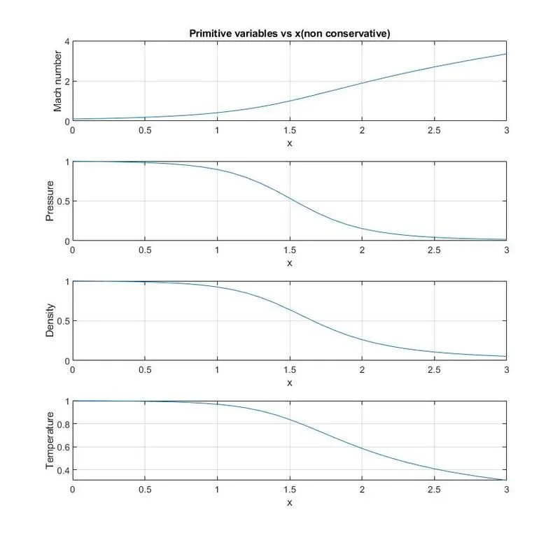
- Steady state distribution of primitive variables inside the nozzle ( NON-CONSERVATIVE FORM )
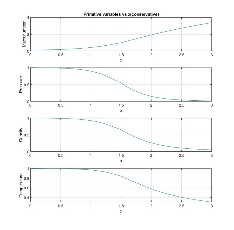
- Steady state distribution of primitive variables inside the nozzle ( CONSERVATIVE FORM )
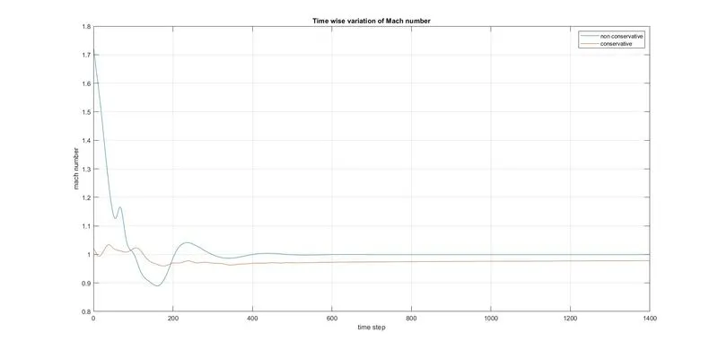
- Time wise variation of Mach number
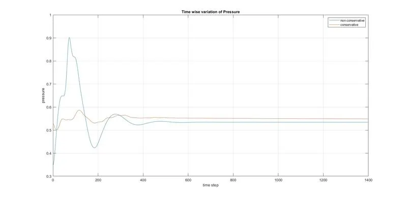
- Time wise variation of Pressure
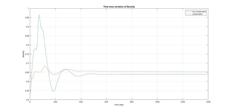
- Time wise variation of Density
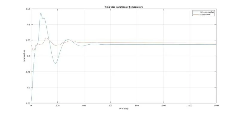
- Time wise variation of Temperature
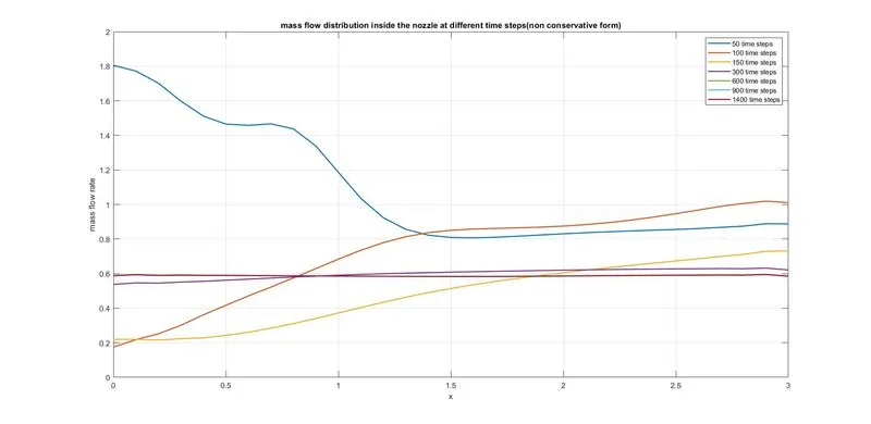
- Variation of Mass flow rate distribution inside the nozzle at different time steps ( NON-CONSERVATIVE FORM )
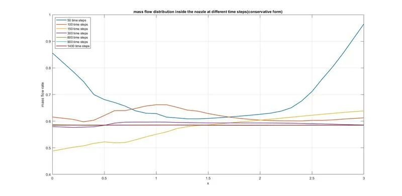
- Variation of Mass flow rate distribution inside the nozzle at different time steps ( CONSERVATIVE FORM )
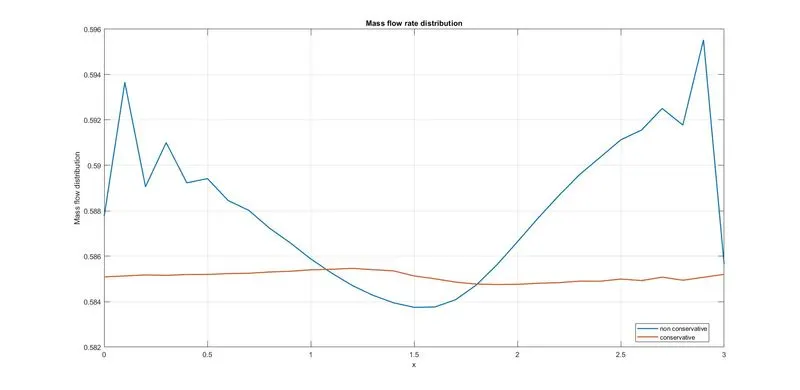
- Comparison of Normalized mass flow rate distribution of both forms
CONCLUSION
- From these graphs we can conclude that Conservative form is far better than Non conservative form.
- From the 'Mass flow rate distribution at different time step' graph and 'Time wise variation of primitive variables' graph we can easily understands that Conservative form become stable faster than the Non-Conservative form.
- It can be observed that at smaller time steps the behaviour of Non-Conservative form shows highly unstable results than the Conservative form.
- It can be observed that after 300 time steps, all the primitive variables and mass flow rate distributions are showing stable results.
- The Macormack method provides quite stable and exact solutions. Because here we are not directly going to next time step. Here we have additional steps, which are predictor step,corrector step and averaging. Then only we updating the solution. And this is the reason why we are getting more stable and exact solutions.