Week 8 - Simulation of a backward facing step in OpenFOAM

In this problem we have to simulate an incompressible-laminar-viscous flow through a backward step geometry by using OpenFOAM.

By checking the solver folder we can understand that icoFoam solver is used to solve this problem.

THE SIMULATION PROCEDURE USING OpenFOAM

1. Open the terminal window. (ctrl+alt+T)
2. Go to tutorial folder by typing 'tut'
3. Go to Incompressible folder by typing 'cd Incompressible/'
4. Go to icoFoam folder by typing 'cd icoFoam/'
5. Inside that, go to cavity folder by typing 'cd cavity/'
6. Copy the cavity folder inside the main folder, to a new folder(cavity_test) inside run folder, So that the offical file of the OpenFOAM remain untouched.('cp -r cavity/ $FOAM_RUN/ cavity_test)
7. Go to the run folder by typing 'run'
8. Open the 'cavity_test' folder. (cd cavity_test)
9. Find out the 'blockMeshDict' script file inside the system folder. (cd system)
10. Open the block mesh file and edit it to specify the doamin and mesh. To open the file, type 'gedit blockMeshDict' in the command window.
11. Find out the 'controlDict' script file and edit it to check the starting time, ending time and dT. (gedit controlDict)
12. Go to 0 folder to edit the initial conditions of velocity and pressure (the files are named as 'U' and 'p') according to the faces of the given domain. (cd ..`rarr`cd 0)
13. After completing whole editing use 'blockMesh' command to generate the mesh and 'checkMesh' to verify it.
14. Then open paraView by typing 'paraFoam'.
15. When it gets open click 'apply' to show the geometry.
16. Plot the velocity profile at 0.085 m from inlet. To do that use 'Plot Over Line' option.
17. Edit the point 1 and point 2 values to 0.085, then only we able to visualise the velocity profile at 0.085.
18. Take screenshot and lock it.

We need to do this for the geometry with grading factor 0.2. So repeat the whole procedure to visualise the velocity profile of the geometry with grading factor 0.2. Inorder to change the grading factor we need to go through the 'blockMeshDict' file.

EDITING 'blockMeshDict' FILE FOR THE 1st CASE ( Grading Factor = 1)

The 'blockMeshDict' file is a script file contains all informations about the geometry.

Open the 'blockMeshDict' file and change the parameters as shown below.

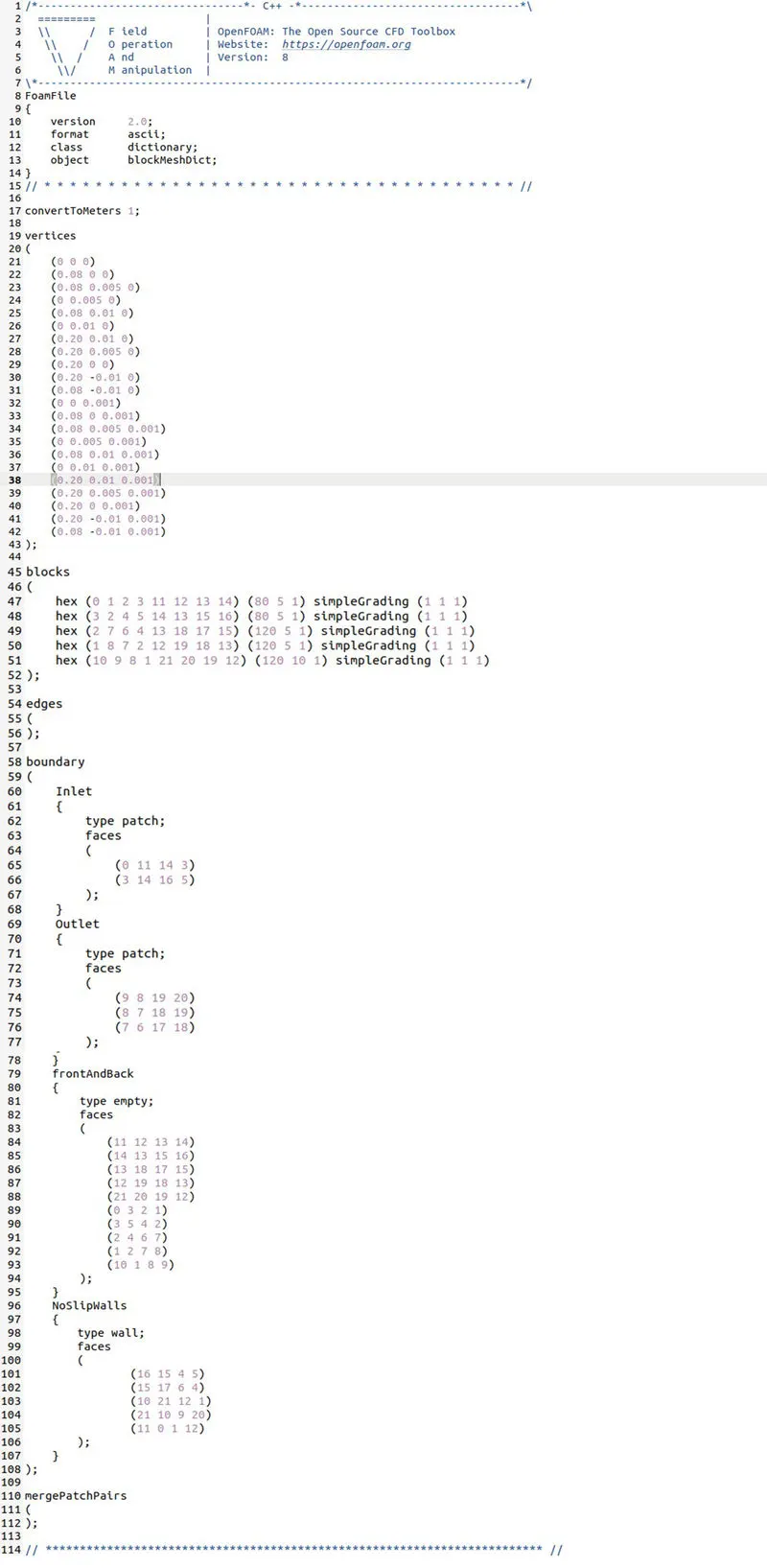
• The portion which includes line number 1 to 7 of the code is known as Header information, which are not executable.
• The portion which includes line number 8 to 16 of the code is known as File identifier, which OpenFOAM reads the type of file its reading. This structure is known as Dictionary format. Which contains a Key and a Value. Here Version is the key and 2.0 is the value. So this is called as Key-Value pair.
• By default OpenFOAM assumes all the geometries are in Meters. So line number 17 ( convertToMeters ) is used to convert all type of length into meters.
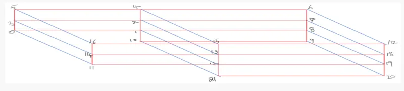
• From the next line onwards (line number 19 to 43) we define the vertices. The vertices are mentioned with x,y and z co-ordinates. For this geometry we have 22 vertices which starts from 0 to 21. And they are listed in order(0 to 21). The vortices of the geometry is shown below.
• The general idea of block mesh is to represent the geometry as a set of blocks. For this geometry we have 5 blocks.
• Here the 5 blocks are defined from line number 45 to 52. The first keyword (hex) defines the type of mesh used, i.e, here it is Hexahedral. The 8 numbers(vertices) with in a bracket define particular blocks. The next 3 numbers within the bracket defines the number of cells (mesh points) along the x,y and z axis. We know that the toal number of cells along x direction is 200 and along y direction is 20. Since we need uniform distribution put number of cells along x axis for first two blocks(1 and 2) as 80, because the length of these two blocks are 0.08 m and put number of cells along y axis as 5 for first 4 blocks(1,2,3 and 4). For 3rd,4th and 5th blocks put number of cells along x axis as 120. For the 5th block put the number of cells along y axis as 10.
• The next keyword 'simpleGrading' tell us about the grading of the cells. It refers to a technique called Mesh stretching. And the three numbers with in the bracket next to the keyword(simpleGrading) defines the grading factors along x,y and z axis. In this case the grading factor is 1. that's why it is mentioned as (0 0 0). Mesh grading is very useful for the computer efficiency. Mesh grading is a factor, which can be defined as the ratio of size of end cell to the size of starting cell.

Grading Factor, f = (Size of end cell) / (Size of starting cell)

• The next step is to defining the boundaries of the geometry. The portion which includes line number 58 to 108 of the code represents the boundary list, which are Inlet, Outlet, Fixed walls( No slip walls ) and Front and Back. Since it is a 3D geometry the boundaries are going to be faces. Each 4 number sets define particular faces of the geometry as shown in the code above. A face is refers to a patch in OpenFOAM. While defining a face of the geometry the order of entering numbers should be in anti-clockwise, because OpenFOAM follows Right Hand Thumb rule.
• Line number 110 to 114 is about the merging of faces and blocks. The keyword 'mergePatchPairs' is used to merging. This option is required when we have more than one block.
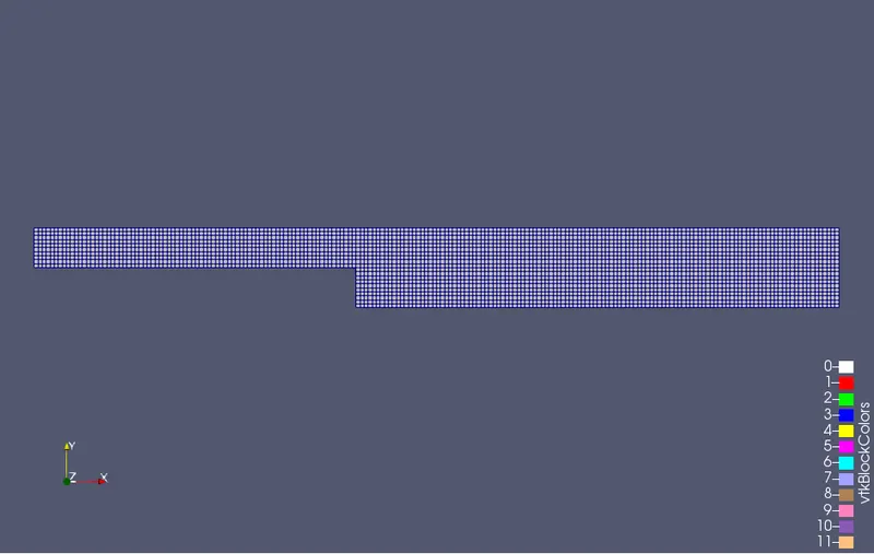
• Finally we get a mesh like this,

• 

EDITING 'controlDict' FILE FOR THE 1st CASE ( Grading Factor = 1)

Open the 'blockMeshDict' file and change the parameters as shown below.

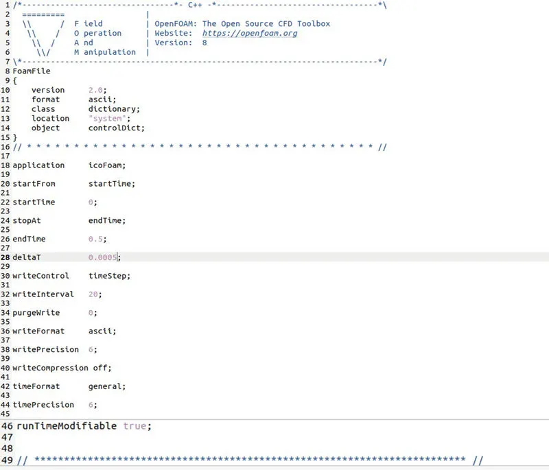
• Like the 'blockMeshDict' file we can see the Header and File identifier portion in this file too.
• 'controlDict' file is also a script file, which includes the detailes of simulation time, dT etc.
• Here we change 'dT' value to 0.005, then only we get appropriate CFL number which less than 1.

EDITING INITIAL CONDITIONS OF VELOCITY AND PRESSURE [U and p] FOR THE BOTH CASES

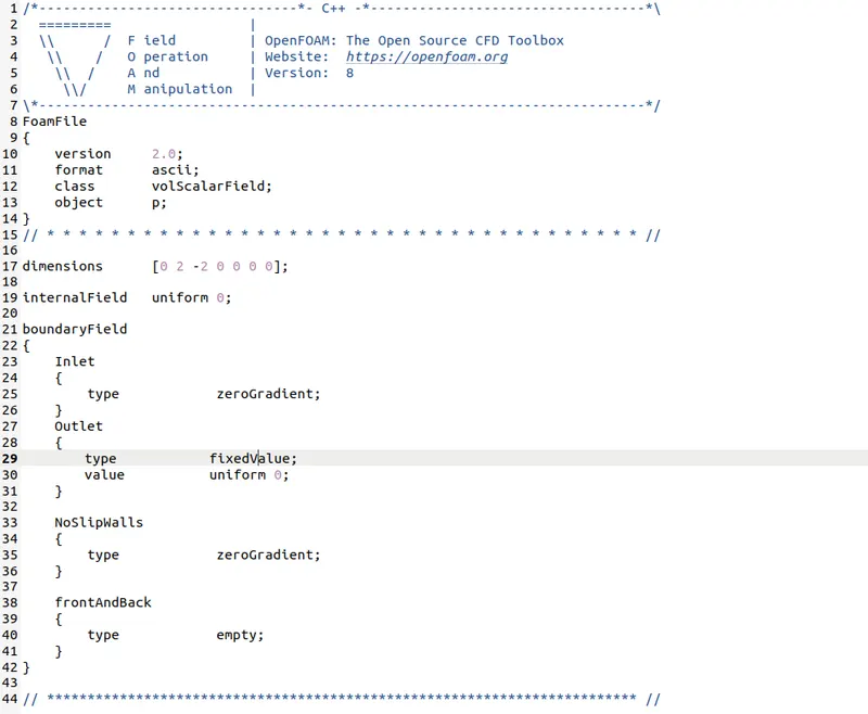
These two files are located in '0' folder. Initially in these two files the boundaries are mentioned with different names. So we need to define the boundaries and their types correctly for these two files. That's all we need to change here. The rest of the details has no changes. Edit the files as shown below,

• Pressure :-

• Velocity :-
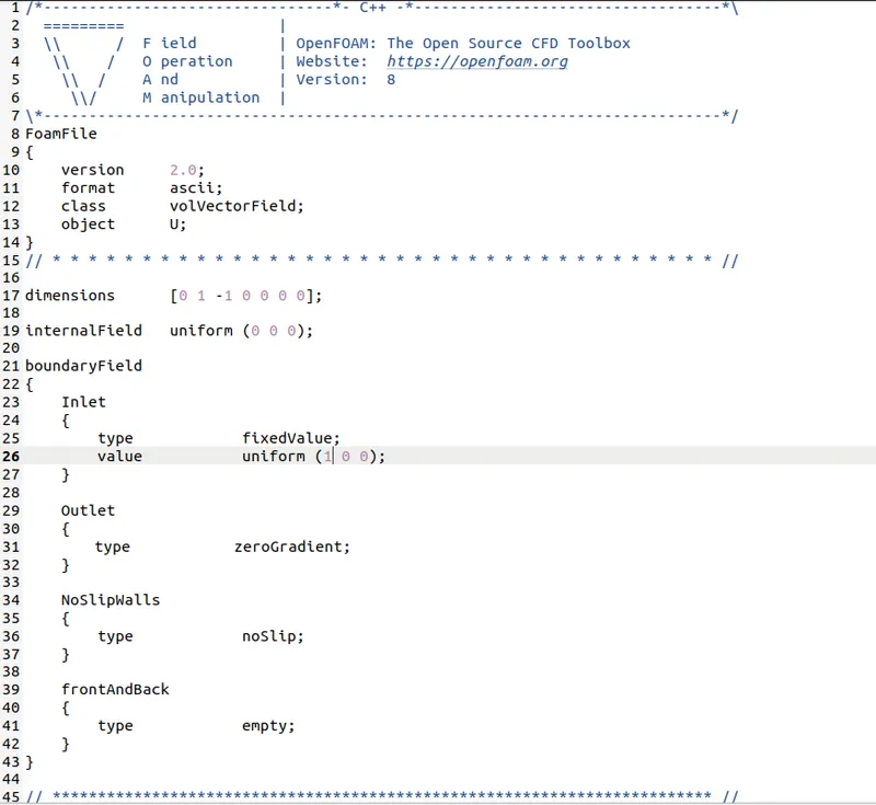
• Here in the inlet we specify the value of velocity(1 m/s). It is mentioned in the line number 26.

EDITING 'blockMeshDict' FILE FOR THE 2nd CASE ( Grading Factor = 0.2 )

Open the 'blockMeshDict' file and change the parameters as shown below.

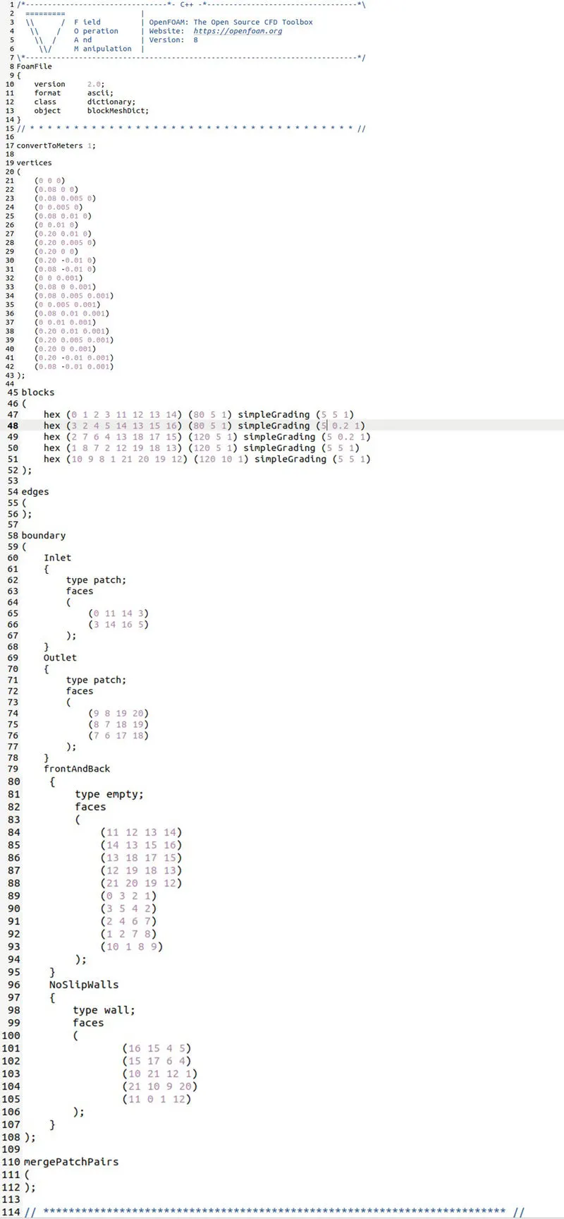
• From this code we can easily understand that the only difference is occuring in the portion where defining the blocks and mesh grading (line number 45 to 52).
• The rest of the code is same as the previous case(grading factor 1).
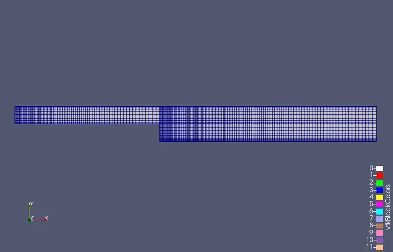
• Here we are simulating flow with grading factor 0.2. And the grading should be finer near the walls( including step walls). So we enter the grading values like this,
• Then we get a mesh grading like this,

EDITING 'controlDict' FILE FOR THE 2nd CASE ( Grading Factor = 0.2)

Open the 'blockMeshDict' file and change the parameters as shown below.

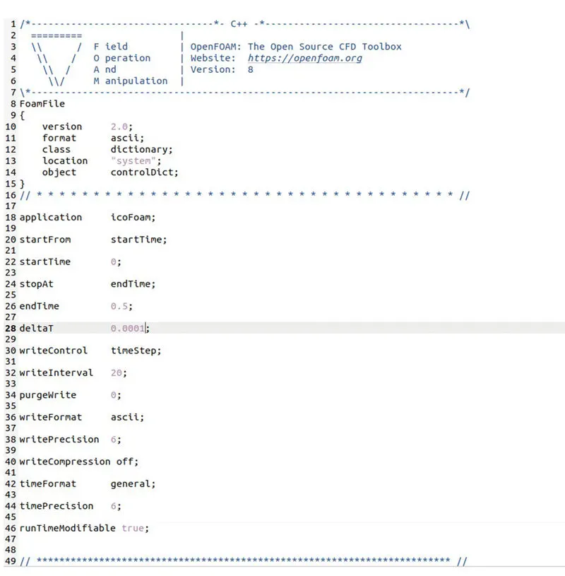
• Here we change 'dT' value to 0.0001, then only we get appropriate CFL number which less than 1.

ParaView PROCEDURES

• Open paraView by typing 'paraFoam' in the terminal window.
• Click on the apply button in the properties section to see the geometry.
• Change the option 'vtkBlockColors' to 'U' or 'p'.( Velocity or Pressure)
• Click the play button to show the Velocity or Pressure distribution over the geometry.
• To plot the velocity profile at 0.085m from inlet, use plot over line option. ( Filters`rarr`Data Analysis`rarr`Plot over line )
• Click on the 'Y axis' option and change the values of point 1 and point 2 to 0.085.
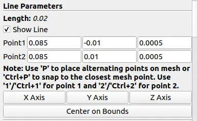
• Uncheck the pressure(p).
• Then click on 'Apply' button to plot the velocity profile at 0.085m from the inlet.

OUTPUTS

• Velocity distribution over the geometry - CASE 1 ( Grading Factor = 1 )

• Cell Data :-

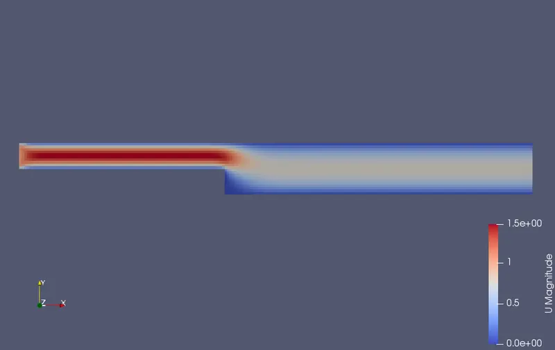
• Point Data :-

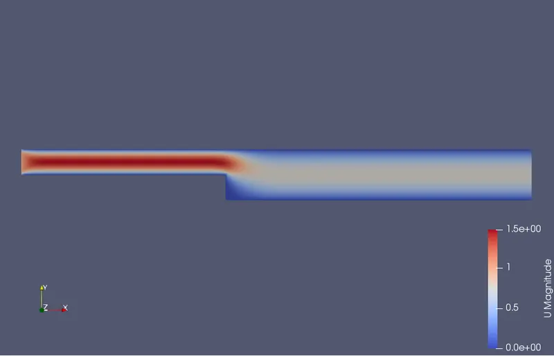
• Pressure distribution over the geometry - CASE 1 ( Grading Factor = 1 )

• Cell Data :-

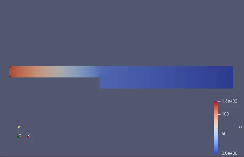
• Point Data :-

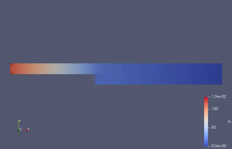
• Velocity distribution over the geometry - CASE 2 ( Grading Factor = 0.2 )

• Cell Data :-

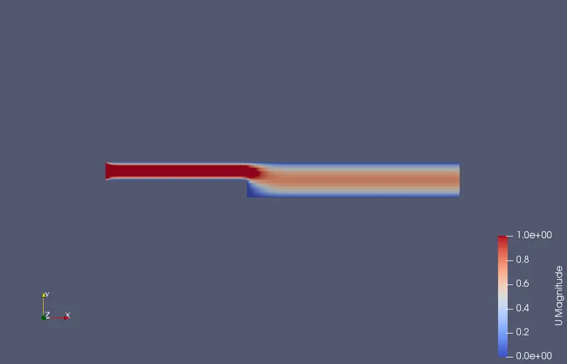
• Point Data :-

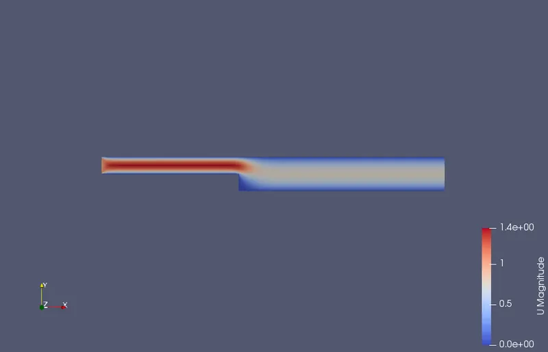
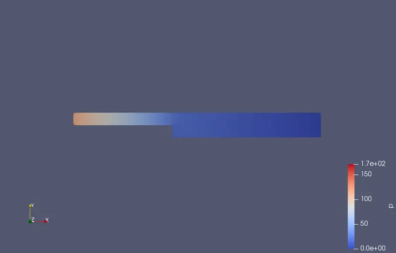
• Pressure distribution over the geometry - CASE 2 ( Grading Factor = 0.2 )

• Cell Data :-

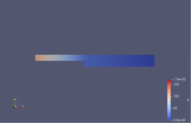
• Point Data :-

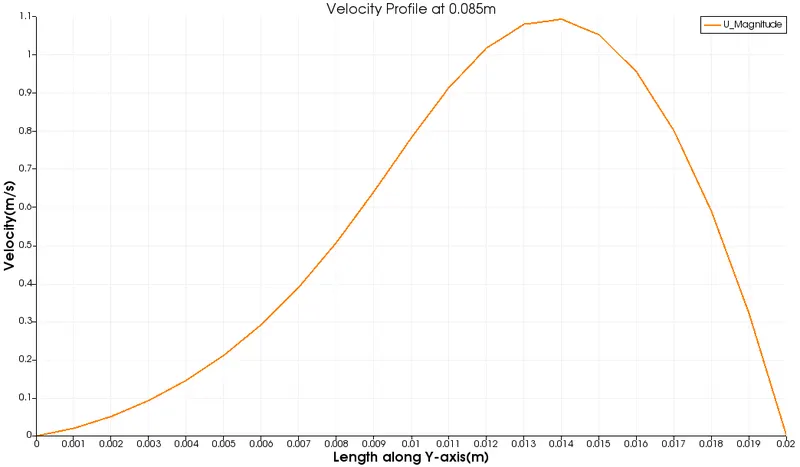
• Velocity profile at 0.085m for CASE 1 ( Grading Factor = 1 )

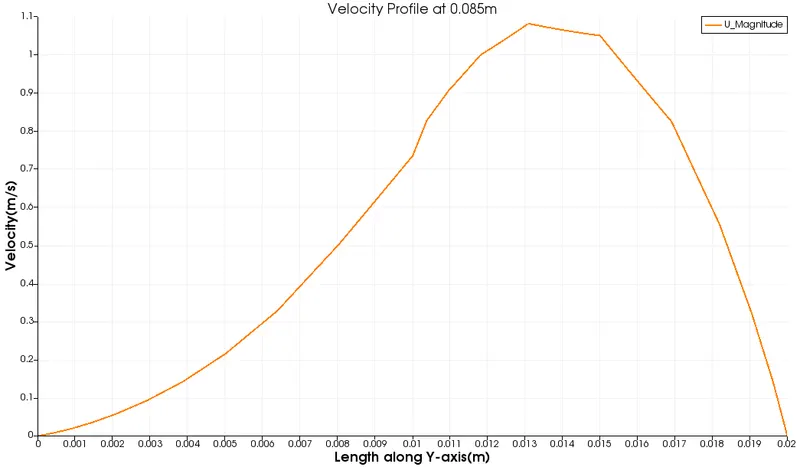
• Velocity profile at 0.085m for CASE 2 ( Grading Factor = 0.2 )

CONCLUSION

From these two velocity profiles we can see that, the velocity profile with grading factor 1 is much smooth and accurate than the other plot( velocity profile with grading factor 0.2 ). So one thing we can say that mesh grading can disrupt out the result. But it isn't incorrect. The velocity profile for the 2nd case isn't much smooth and accurate because of its mesh grading.

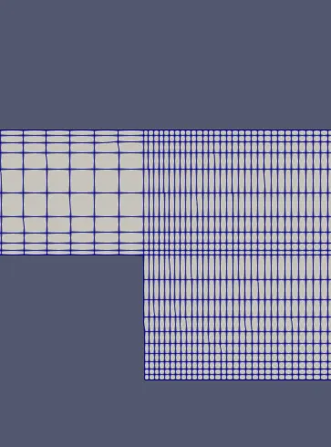
From the above picture we can easily understand that the mesh is finer along x axis, whereas very coarse along y axis. That's why the velocity profile doesn't look good. Because we are plotting the velocity at 0.085m from inlet versus length along Y-axis.

From these two graph we can understand that the velocity at wall is close to 0, at the middle section the velocity reaches maximum( near 1.1 m/s ).