Week 5.1 - Mid term project - Solving the steady and unsteady 2D heat conduction problem
In this problem we are trying to solve the 2D heat conduction equation in both steady state and transient state by explicit and implicit method. Here we are solving the equation with the help of iterative solvers. In steady state approach we employ iterative solvers to solve the equation. In transient state, we employ iterative solvers to solve the equation only in implicit method. Iterative solvers are not necessary to solve the equation by explicit method. Because in explicit method all values are known to find the unknown.
There are 3 Iterative solvers
- Jacobi Method
- Gauss Seidel Method
- Successive Over Relaxation(SOR)
- Explicit Method
Explicit methods calculate the state of system at a later time from the state of the system at the current time.
- Implicit Method
Implicit methods calculate the state of system at a later time from the state of system at both the current time and later time.
Here the domain is a unit square.
Boundary Conditions
Left Boundary = 400K
Right Boundary = 800K
Top Boundary = 600K
Bottom Boundary = 900K
Take average of the adjacesnt points along x and y directions to find the temperatures at the corners.
i.e,
t(1,1)=500K
t(1,10)=650K
t(10,1)=700K
t(10,10)=850K
Here we taking the temperatures for the inner nodes as 300K.
Iterative Solvers
- Jacobi Method
In this method the values at the (n+1)th iteration is calculated using old guess values at (n)th iteration.
- Gauss Seidal Method
In this method the values at the (n+1)th iteration is calculated using both old guess values at (n)th iteration and updated values at the (n+1) iteration which is overwritten.
- SOR
It is kind of an enhanced iterative solver, which can be used in both Jacobi or Gauss Seidal method to improve the performance. Here we have a new term called Relaxation factor(`omega`).
When `omega` is between 0-1, it is called under relaxed state.
When `omega>1`, it is called over relaxed state.
2D Heat Conduction Equation
`(delT)/(delt)=alpha.((del^2T)/(delx^2)+(del^2T)/(dely^2))`
Here the time derivative term is hyperbolic in nature. So it can be discretized using forward difference scheme. The spacial tems are elliptic in nature which can be discretized using central differene scheme.
Solving using Steady state approach
Steady state where the properties does not change with respect to time.
So, here the time derivative time will be zero.
Then Steady state 2D heat conduction equation will be,
`(del^2T)/(delx^2)+(del^2T)/(dely^2)=0`
Discretizing using CDS,
`(T(i-1,j)-2T(i,j)+T(i+1,j))/(Deltax^2)+(T(i,j-1)-2T(i,j)+T(i,j+1))/(Deltay^2)=0`
On further simplification, we get
`T(i,j)=1/k[((T(i-1,j)+T(i+1,j))/(Deltax^2))+((T(i,j-1)+T(i,j+1))/(Deltay^2))]`
Where, `k=(2(Deltax^2+Deltay^2))/(Deltax^2.Deltay^2)`
- Equation for Steady state-Jacobi method
`T(i,j)=1/k[((Told(i-1,j)+Told(i+1,j))/(Deltax^2))+((Told(i,j-1)+Told(i,j+1))/(Deltay^2))]`
- Equation for Steady state-Gauss Seidal method
`T(i,j)=1/k[((T(i-1,j)+Told(i+1,j))/(Deltax^2))+((T(i,j-1)+Told(i,j+1))/(Deltay^2))]`
- Equation for Steady state-SOR method
`T(i,j)=Told.(1-omega)+omega.T_(GS)`
Where `T_(GS)` is the T obtained from steady state Gauss Seidal method.
Solving using Transient state approach
Here the equation is,
`(delT)/(delt)=alpha.((del^2T)/(delx^2)+(del^2T)/(dely^2))`
Discretizing,
`(T(i,j)^(n+1)-T(i,j)^n)/(Deltat)=alpha.[(T(i-1,j)-2T(i,j)+T(i+1,j))/(Deltax^2)+(T(i,j-1)-2T(i,j)+T(i,j+1))/(Deltay^2)]`
- Equation for Transient state Explicit method
`(T(i,j)^(n+1)-T(i,j)^n)/(Deltat)=alpha.[(T(i-1,j)-2T(i,j)+T(i+1,j))/(Deltax^2)+(T(i,j-1)-2T(i,j)+T(i,j+1))/(Deltay^2)]^n`
On further simplification, we get
`T(i,j)^(n+1)=T(i,j)^n+(k1.[T(i-1,j)-2T(i,j)+T(i+1,j)]^n)+(k2.[T(i,j-1)-2T(i,j)+T(i,j+1)]^n)`
Where,
`k1=(alphaDeltat)/(Deltax^2)` and `k2=(alphaDeltat)/(Deltay^2)`
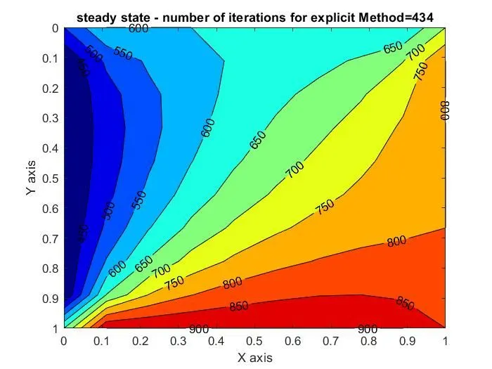
In this case it is not necessary to use the iterative solvers. Because we know all the terms on the RHS of the equation, So we can get the answers directly.
CFL Number
The Courant number can be used in Computational Fluid Dynamics (CFD) simulations to evaluate the time step requirements of a transient simulation for a given mesh size and flow velocity and is linked to the Courant–Friedrichs–Lewy (CFL) stability condition of numerical schemes.
Here CFL number can be calculated with the formula that mentioned below,
`CFL=k1+k2`
Stability Criteria for Explicit diffusion problem
CFL number should be less than or equal to 0.5
`CFL<=0.5`
When CFL number becomes greater than 0.5 the solution gets unstable.
- Equation for Transient state Implicit method
`(T(i,j)^(n+1)-T(i,j)^n)/(Deltat)=alpha.[(T(i-1,j)-2T(i,j)+T(i+1,j))/(Deltax^2)+(T(i,j-1)-2T(i,j)+T(i,j+1))/(Deltay^2)]^(n+1)`
By rearranging,
`T(i,j)^(n+1)=T(i,j)^n+(k1.[T(i-1,j)-2T(i,j)+T(i+1,j)]^(n+1))+(k2.[T(i,j-1)-2T(i,j)+T(i,j+1)]^(n+1))`
Where,
`k1=(alphaDeltat)/(Deltax^2)` and `k2=(alphaDeltat)/(Deltay^2)`
On further simplification, we get
`T(i,j)^(n+1)=1/(1+2.k1+2.k2)[T(i,j)^n+k1[T(i-1,j)+T(i+1,j)]^(n+1)+k2[T(i,j-1)+T(i,j+1)]^(n+1)]`
Equation used in MATLAB program
- Equation for Transient state Explicit method
`T(i,j)^(n+1)=Told(i,j)^n+(k1.[Told(i-1,j)-2Told(i,j)+Told(i+1,j)]^n)+(k2.[Told(i,j-1)-2Told(i,j)+Told(i,j+1)]^n)`
- Equation for Transient state-Implicit Jacobi method
`T(i,j)^(n+1)=1/(1+2.k1+2.k2)[T_(prev)(i,j)^n+k1[Told(i-1,j)+Told(i+1,j)]^(n+1)+k2[Told(i,j-1)+Told(i,j+1)]^(n+1)]`
- Equation for Transient state-Implicit Gauss Seidal method
`T(i,j)^(n+1)=1/(1+2.k1+2.k2)[T_(prev)(i,j)^n+k1[T(i-1,j)+Told(i+1,j)]^(n+1)+k2[T(i,j-1)+Told(i,j+1)]^(n+1)]`
- Equation for Transient state-Implicit SOR method
`T(i,j)=Told.(1-omega)+omega.T_(GS)`
Where `T_(GS)` is the T obtained from transient state-Implicit Gauss Seidal method.
MATLAB PROGRAM CODE
- Steady State
clear all
close all
clc

%solving steady state 2D heat coduction equation using iterative solvers
%(d^2T/dx^2)+(d^2T/dy^2)=0

%initializing variables
%length of the domain is 1

%number of grid points in x direction
nx=10;
%number of grid points in y direction
ny=10;

%initializing temperature array
t=ones(nx,ny);

%top side
t(1,1:ny)=600;
%bottom side
t(nx,1:ny)=900;
%left side
t(1:nx,1)=400;
%right side
t(1:nx,ny)=800;
%left upper node
t(1,1)=500;
%right upper node
t(1,10)=700;
%left lower node
t(10,1)=650;
%right lower node
t(10,10)=850;
%inner nodes
t(2:nx-1,2:ny-1)=300;

x=linspace(0,1,nx);
y=linspace(0,1,ny);

%grid size
dx=x(2)-x(1);
dy=y(2)-y(1);

%mesh grid
[X, Y]=meshgrid(x,y);

k=(2*((dx^2)+(dy^2)))/((dx^2)*(dy^2));

%copying values of t
told_j=t;
told_gs=t;
told_sor=t;

%omega(relaxation factor)
w=1.1;

%tolerance
tol=1e-4;

error=5;

method = 1; %( 1.Jacobi 2.GS 3.SOR)

jacobi_iter=1;
gs_iter=1;
sor_iter=1;


%steady state-Jacobi method

if(method==1)
    while(error>tol)
        for i=2:nx-1
            for j=2:ny-1
                term1=(told_j(i-1,j)+told_j(i+1,j))/(dx^2);
                term2=(told_j(i,j-1)+told_j(i,j+1))/(dy^2);
                t(i,j)=(term1+term2)/k;
            end
        end
        error=max(max(abs(told_j-t)));
        told_j=t;
        jacobi_iter=jacobi_iter+1;
    end

figure(1)
contourf(x,y,t,'showtext','on')
set(gca,'YDIR','reverse')
colormap('jet')
xlabel('X axis')
ylabel('Y axis')
title(sprintf('steady state - number of iterations for JACOBI Method=%d',jacobi_iter))
end


%steady state-Gauss Seidal method
if(method==2)
        while(error>tol)
        for i=2:nx-1
            for j=2:ny-1
                term1=(t(i-1,j)+told_gs(i+1,j))/(dx^2);
                term2=(t(i,j-1)+told_gs(i,j+1))/(dy^2);
                t(i,j)=(term1+term2)/k;
            end
        end
        error=max(max(abs(told_gs-t)));
        told_gs=t;
        gs_iter=gs_iter+1;
        end

figure(2)
contourf(x,y,t,'showtext','on')
set(gca,'YDIR','reverse')
colormap('jet')
xlabel('X axis')
ylabel('Y axis')
title(sprintf('steady state - number of iterations for GS Method=%d',gs_iter))
end


%steady state-SOR method

if(method==3)
        while(error>tol)
        for i=2:nx-1
            for j=2:ny-1
                term1=(t(i-1,j)+told_sor(i+1,j))/(dx^2);
                term2=(t(i,j-1)+told_sor(i,j+1))/(dy^2);
                t(i,j)=(term1+term2)/k;
                t(i,j)=(told_sor(i,j)*(1-w))+(w*t(i,j));
            end
        end
        error=max(max(abs(told_sor-t)));
        told_sor=t;
        sor_iter=sor_iter+1;
        end

figure(3)
contourf(x,y,t,'showtext','on')
set(gca,'YDIR','reverse')
colormap('jet')
xlabel('X axis')
ylabel('Y axis')
title(sprintf('steady state - number of iterations for SOR Method=%d',sor_iter))
end- Transient state - Explicit method
clear all
close all
clc

%solving transient state 2D heat coduction equation
%dT/dt=alpha*(d^2T/dx^2)+(d^2T/dy^2)

%initializing variables
%length of the domain is 1

%number of grid points in x direction
nx=10;
%number of grid points in y direction
ny=10;

%initializing temperature array
t=ones(nx,ny);

%top side
t(1,1:ny)=600;
%bottom side
t(nx,1:ny)=900;
%left side
t(1:nx,1)=400;
%right side
t(1:nx,ny)=800;
%left upper node
t(1,1)=500;
%right upper node
t(1,10)=700;
%left lower node
t(10,1)=650;
%right lower node
t(10,10)=850;
%inner nodes
t(2:nx-1,2:ny-1)=300;

x=linspace(0,1,nx);
y=linspace(0,1,ny);

%grid size
dx=x(2)-x(1);
dy=y(2)-y(1);

nt=1400;

%time step
dt=0.001;

%mesh grid
[X, Y]=meshgrid(x,y);


%copying values of t
told=t;


%tolerance
tol=1e-4;

error=5;

alpha=1.4; %thermal diffusivity
k1=(alpha*dt)/(dx^2);
k2=(alpha*dt)/(dy^2);
cfl=k1+k2; %CFL number

explicit_iter=1;

        for k=1:nt                 %time loop
            while(error>tol)       %convergence loop
            for i=2:nx-1           %space loop
                for j=2:ny-1
                    term1=told(i,j);
                    term2=(k1*((told(i-1,j))-(2*told(i,j))+(told(i+1,j))));
                    term3=(k2*((told(i,j-1))-(2*told(i,j))+(told(i,j+1))));
                    t(i,j)=term1+term2+term3;
                end
            end
            error=max(max(abs(told-t)));
            told=t;
            explicit_iter=explicit_iter+1;
            end
        end

    figure(1)
    contourf(x,y,t,'showtext','on')
    set(gca,'YDIR','reverse')
    colormap('jet')
    xlabel('X axis')
    ylabel('Y axis')
title(sprintf('steady state - number of iterations for explicit Method=%d',explicit_iter))- Transient state - Implicit method
clear all
close all
clc

%solving transient state 2D heat coduction equation using iterative solvers
%dT/dt=alpha*(d^2T/dx^2)+(d^2T/dy^2)


%initializing variables
%length of the domain is 1

%number of grid points in x direction
nx=10;
%number of grid points in y direction
ny=10;

%initializing temperature array
t=ones(nx,ny);

%top side
t(1,1:ny)=600;
%bottom side
t(nx,1:ny)=900;
%left side
t(1:nx,1)=400;
%right side
t(1:nx,ny)=800;
%left upper node
t(1,1)=500;
%right upper node
t(1,10)=700;
%left lower node
t(10,1)=650;
%right lower node
t(10,10)=850;
%inner nodes
t(2:nx-1,2:ny-1)=300;

x=linspace(0,1,nx);
y=linspace(0,1,ny);

%grid size
dx=x(2)-x(1);
dy=y(2)-y(1);

nt=1400;

%time step
dt=0.01;

%mesh grid
[X, Y]=meshgrid(x,y);


%copying values of t
told_j=t;
told_gs=t;
told_sor=t;
t_prev=t;


%tolerance
tol=1e-4;

error=5;

alpha=1.4; %thermal diffusivity
k1=(alpha*dt)/(dx^2);
k2=(alpha*dt)/(dy^2);
cfl=k1+k2;


jacobi_iter=1;
gs_iter=1;
sor_iter=1;

method = 1; %( 1.Jacobi 2.GS 3.SOR)

w=1.4; %relaxation factor


%transient state-implicit Jacobi method

if(method==1)
        for m=1:nt                      %time loop
            error=5;
            while(error>tol)            %convergence loop
                for i=2:nx-1            %space loop
                    for j=2:ny-1

                        term1=(1/(1+(2*k1)+(2*k2)));
                        term2=k1*term1;
                        term3=k2*term1;
                        h=told_j(i-1,j)+told_j(i+1,j);
                        v=told_j(i,j-1)+told_j(i,j+1);
                        t(i,j)=(t_prev(i,j)*term1)+(h*term2)+(v*term3);

                    end
                end
            error=max(max(abs(told_j-t)));
            told_j=t;
            jacobi_iter=jacobi_iter+1;
            end
            t_prev=t;
        end

figure(1)
contourf(x,y,t,'showtext','on')
set(gca,'YDIR','reverse')
colormap('jet')
xlabel('X axis')
ylabel('Y axis')
title(sprintf('transient state(Implicit) - number of iterations for Jacobi Method=%d',jacobi_iter))
end


%transient state-implicit Gauss Seidal Method

if(method==2)
        for m=1:nt
            error=5;
            while(error>tol)
                for i=2:nx-1
                    for j=2:ny-1

                        term1=(1/(1+(2*k1)+(2*k2)));
                        term2=k1*term1;
                        term3=k2*term1;
                        h=t(i-1,j)+told_gs(i+1,j);
                        v=t(i,j-1)+told_gs(i,j+1);
                        t(i,j)=(t_prev(i,j)*term1)+(h*term2)+(v*term3);

                    end
                end
            error=max(max(abs(told_gs-t)));
            told_gs=t;
            gs_iter=gs_iter+1;
            end
            t_prev=t;
        end

figure(2)
contourf(x,y,t,'showtext','on')
set(gca,'YDIR','reverse')
colormap('jet')
xlabel('X axis')
ylabel('Y axis')
title(sprintf('transient state(Implicit) - number of iterations for GS Method=%d',gs_iter))
end


%transient state-implicit SOR method

if(method==3)
        for m=1:nt
            error=5;
            while(error>tol)
                for i=2:nx-1
                    for j=2:ny-1

                        term1=(1/(1+(2*k1)+(2*k2)));
                        term2=k1*term1;
                        term3=k2*term1;
                        h=t(i-1,j)+told_sor(i+1,j);
                        v=t(i,j-1)+told_sor(i,j+1);
                        t(i,j)=(t_prev(i,j)*term1)+(h*term2)+(v*term3);
                        t(i,j)=(told_sor(i,j)*(1-w))+(w*t(i,j));

                    end
                end
            error=max(max(abs(told_sor-t)));
            told_sor=t;
            sor_iter=sor_iter+1;
            end
            t_prev=t;
        end

figure(3)
contourf(x,y,t,'showtext','on')
set(gca,'YDIR','reverse')
colormap('jet')
xlabel('X axis')
ylabel('Y axis')
title(sprintf('transient state(Implicit) - number of iterations for SOR Method=%d',sor_iter))
end
EXPLANATION OF CODES
- [X, Y]=meshgrid(x,y)
returns 2-D grid coordinates based on the coordinates contained in vectors x and y. X is a matrix where each row is a copy of x, and Y is a matrix where each column is a copy of y. The grid represented by the coordinates X and Y has length(y) rows and length(x) columns. - If ( If - end ) command evaluates an expression, and executes a group of statements when the expression is true. An expression is true when its result is nonempty and contains only nonzero elements. Otherwise, the expression is false.
- While loop ( while - end ) evaluates an expression, and repeats the execution of a group of statements in a loop while the expression is true. An expression is true when its result is nonempty and contains only nonzero elements. Otherwise, the expression is false. Here While loop is the convergence loop.
- contourf(x,y,t) command creates a filled contour plot specifies the x and y coordinates for the values in t.
- showtext command used to displays the contour line labels.
- on is used to display the values along the contour lines.
- set(gca,'YDIR','reverse') command is used to reverse the y values. i.e, instead of showing the y axis as 0 to 1, this command displays in reverse order. i.e, it displays the values on y axis as 1 to 0.
- colormap('jet') command returns the jet colormap for the current figure.
- sprintf command used to format data into string or character vector.
OUTPUT
- Graph
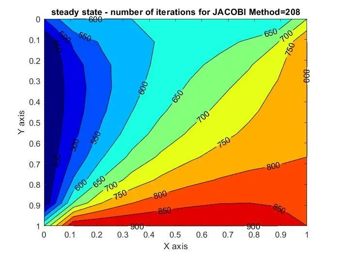
- STEADY STATE - JACOBI METHOD
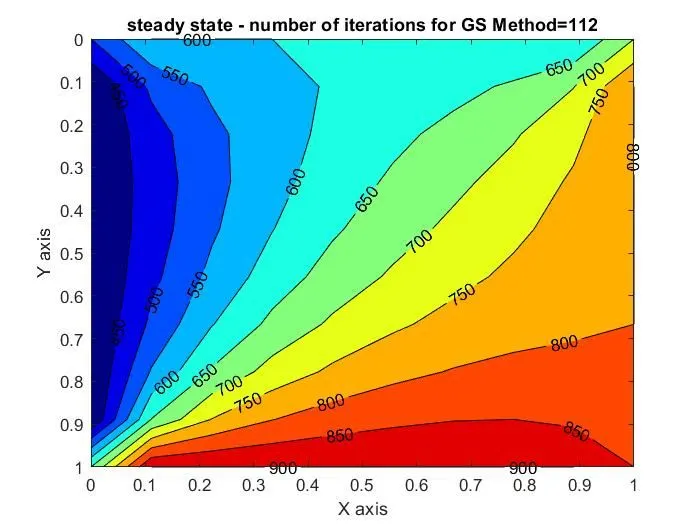
- STEADY STATE - GAUSS SEIDAL METHOD
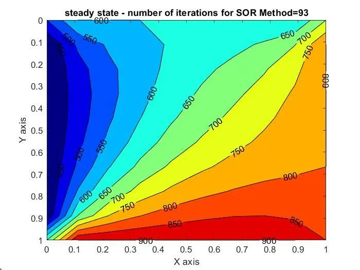
- STEADY STATE - SOR METHOD
- TRANSIENT STATE - EXPLICIT METHOD
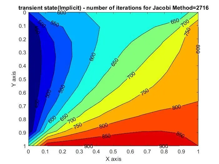
- TRANSIENT STATE - IMPLICIT JACOBI METHOD
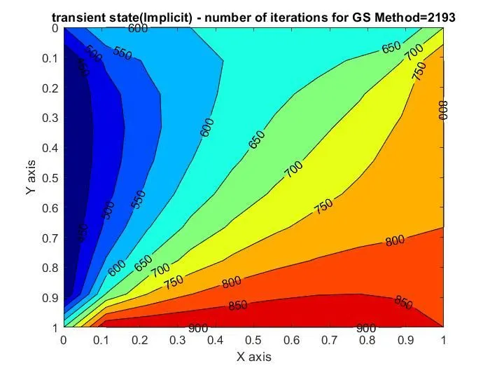
- TRANSIENT STATE - IMPLICIT GAUSS SEIDAL METHOD
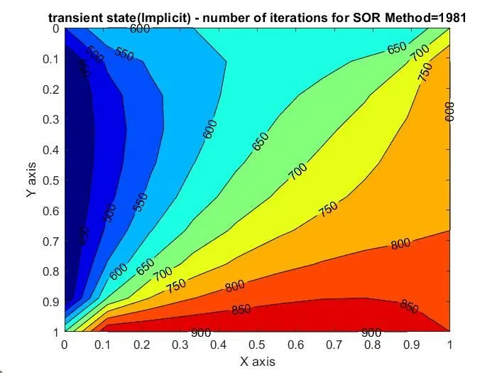
- TRANSIENT STATE - IMPLICIT SOR METHOD
- CONCLUSION
Steady State approach
|
Iterative solver |
Number of Iterations |
| Jacobi | 208 |
| Gauss Seidal | 112 |
| SOR | 93 |
Transient State approach (Implicit method )
|
Iterative solver |
Number of Iterations |
| Jacobi | 2716 |
| Gauss Seidal | 2193 |
| SOR | 1981 |
Iterations for Jacobi > Gauss Seidal > SOR.
From the above plots and tables we can see that the SOR method has the fastest convergence rate, followed by Gauss Seidal and Jacobi methods. So we can conclude that SOR method is the most effective method among the 3 Iterative solvers since it converges the solution for a lesser number of Iterations. Hence SOR method takes less time than the other two methods. SOR is mainly depends on the value of `omega`. If an appropriate value is chosen for `omega`, then the solution converges faster, otherwise the solution may take longer to converge.