Week 9 - FVM Literature Review
-
- Finite Volume Method:
- Step 1: The domain under study is divided into a number of finite-sized subdomains (control volumes). The shape of these control volumes is completely arbitrary and no assumptions are made about it. Each domain represents a finite number of grid points.
- Step 2: Governing Differential equations are integrated over each sub-domain to obtain Integral equations.
- Step3: The integrals are evaluated using function values at the nodes (usually taken as the geometric centers of control volumes). The results are expressed in the form of algebraic quantities at grid points. We require interpolation functions for this purpose.
- The main advantage of FVM is that it carries the physical meaning of conservation with it.
- Major Differences between FVM and FDM:
- In FDM, The domain is divided into a number of grid points. Implementation is easier because of the use of the Taylor series for discretization. However, this very fact makes it difficult to handle complex geometries in FDM. It is difficult to handle the grids that are not aligned along x, y, or z.
- In FVM the domain is divided into control volumes. the shape of these control volumes is completely arbitrary and no assumptions are made. Thus, can handle complex geometry in a better manner as compared to FDM.
- The physical sense of conservation is represented better in FVM as compared to FDM which makes it popular
- Coding for FVM is more complex compared to that of FDM.
- Need of Interpolation Scheme and Flux Limiters:
- Interpolation Scheme:
- In order to obtain the integral over each discrete grid point (node or centre of control volume), we require an approximate distribution of properties between nodal points. That is why there is a need for interpolation Schemes. In FVM the interpolation function is used only for evaluating the integral and is not required after that for obtaining any data. Hence FVM is flexible in using various interpolation schemes for the solution of integral.
- Different interpolation schemes used are as follows:
- Central Differencing, upwind, hybrid and power law.
- Higher-order schemes such as QUICK.
- higher-order schemes can give rise to undershoots and overshoots i.e oscillations in solutions.
- Flux Limiters:
- in order to achieve oscillation-free solutions, we use TVD schemes that apply Flux limiter. It addresses the issue of undesirable oscillations by limiting the range of possible values of the additional convective flux.
- The choice of limiter function decides the order of the scheme and its boundedness properties.
- Interpolation Scheme:
- Example:
- The governing differential equation of 1D steady-state heat conduction equation is given as :
- `(d(k(dT)/dx))/(dx)+S=0` where S is the source term.
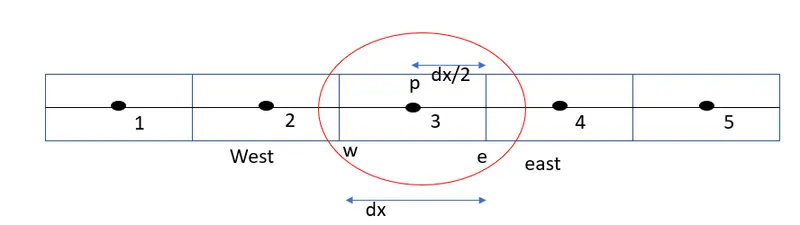
- Integrating the governing differential equation
- `int_w^e(d(k(dT)/dx))/(dx)dV+int_w^eSdV=0`
- `int_w^e(d(k(dT)/dx))/(dx)dV+int_w^eSdV=0`
- `alpha_eA(delT)/(delx_e)-alpha_wA(delT)/(delx_w)+SdV=0`
- using central differencing interpolation scheme we obtain
- `alpha_eA[(T_e-T_p)/(Deltax)]-alpha_wA[(T_e-T_p)/(Deltax)]+SdV=0`
- Now the above equation can be solved using suitable methods.
- Finite Volume Method: