Week 7 - Simulation of a 1D Super-sonic nozzle flow simulation using Macormack Method

• Physics of the problem:

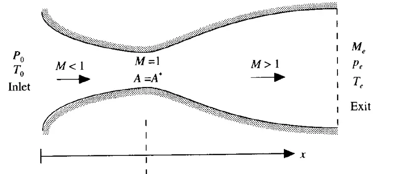
• • The flow expands isentropically to supersonic speeds at the nozzle exit.
  • flow is subsonic in the convergent section, sonic in the throat section, and supersonic in the divergent section.
  • Although the flow through the nozzle is 2D we assume that properties vary only along the x-direction. such type of flow is called quasi-1D flow.

• Setup for the current problem:
  
  • Derivation of governing equations: In this case, we cannot directly apply the governing equations for 1D flow due to the assumption of quasi 1D flow ( which changes the physics as actual flow is in 2D). so we have to derive the equations for the control volume specific to our problem
  • Set up Numerical Scheme
  • Calculation of time step
  • Boundary conditions
  • Initial Conditions

Derivation of Governing Equations

Conservative and Nonconservative form of governing equations:

Continuity Equation

the integral form of governing equations

`del /(delt)int int int rho dAA+int int rho V.ds=0` ............(1)

now, `del/(delt) int int int rho dAA = del/(delt) (rho A dx)`

and `int int rho Vds = -rhoVA+(rho+drho)(V+dV)(A+dA)`

`= -rhoVA + rhoVA + rhoVdA+rhodVA+rhodVdA +drhoVA+drhoVdA+drhodVA+ drhodVdA`

as dx is small all derivative products can be cancelled and we are finally left with

`int int rhoVds = d(rhoVA)`

thus equation 1 becomes

`(del rhoAdx) /(delt)+d (rho AV)=0`

dividing by dx on both sides,

`(del (rhoA))/(delt)+(del(rhoAV))/(delx)=0` .............. (2)

equation (2) is PDE form of continuity equation for unsteady, quasi-1D flow in conservation form.

in order to obtain the non-conservative form simply expand the second term of equation 2.

`(del(rhoA))/(delt)+V(del(rhoA))/(delx)+rhoA(delV)/(delx)=0`............... (3)

equation (3) is the nonconservative form of continuity equation.

Momentum Equation

integral form of x-momentum for an inviscid flow with no body forces

`del/(delt) int int int (rhou)dAA+ int int (rhouV)ds = - int int pds` ...........................(4)

where, `del/(delt)int int int (rho u )dAA = (del ( rhoVAdx))/(delt)`

also, the second term of equation 4 reduces to equation below by performing similar opration as in case of continuity.

`int int rho u Vds = d(rhoAV^2)`

and `int int pds = -PA+(P+dP)(A+dA)-2P((dA)/2) = A.dp`

the term `-2P((dA)/2)` appears due to the inclined faces of the control volume.

after substitution equation 4 becomes to

`(del(rhoVAdx))/(delt) + d(rhoAV^2)=-Adp`

dividing both sides by dx

`(del(rhoVA))/(delt) + (del(rhoAV^2))/(delx) = -A (delP)/(delx)`----------------(5)

Equation 5 is the conservative form of momentum equation

to obtain the nonconservative form of momentum equation expand the first and second term of equation 5

we get, `rhoA (delV)/(delt) + V(del(rhoA))/(delt)+rhoAV(delV)/(delx)+V[(del(rhoAV))/(delx)] = -A(delP)/(delx)`

`rhoA (delV)/(delt) + V(del(rhoA))/(delt)+rhoAV(delV)/(delx)+V[V(del(rhoA))/(delx)+rhoA(delV)/(delx)] = -A(delP)/(delx)`

`rhoA (delV)/(delt) + V[(del(rhoA))/(delt)+V(del(rhoA))/(delx)+rhoA(delV)/(delx)]+rhoAV(delV)/(delx) = -A(delP)/(delx)`

the term in square bracket represents continuity equation and thus can be equated to zero and dividing both sides by A we get

`rho (delV)/(delt) +rhoV(delV)/(delx) = -(delP)/(delx)`............................... (6)

Equation 6 is the non-conservative form of momentum equation

Energy Equation

the integral form of energy equation:

`del/(delt) int intint rho(e+V^2/2)dAA+intintrho(e+V^2/2)V.ds = -int int (p.V)ds`

using similar procedure as in above equation can be reduced to

`(del[rho(e+V^2/2)Adx])/(delt)-d[rho(e+V^2/2)VA]=-d(pAV)`

dividing both sides by dx we get

`(del[rho(e+V^2/2)A])/(delt)+(del[rho(e+V^2/2)VA])/(delx)=-(del(pAV))/(delx)`............(7`

this is the conservation form of the energy equation.

multiple equation (5) by V we get

`(del(rho(V^2/2)A))/(delt) + (del(rhoA(V^3/2)))/(delx) = -AV (delP)/(delx)``

subtracting this equation from equation (7) we get

`(del[rhoeA])/(delt)+(del[rhoeVA])/(delx)=-p(del(AV))/(delx)`

now multiplying continuity equation by e we get

`e(del (rhoA))/(delt)+e(del(rhoAV))/(delx)=0` subtracting from above equation we get

`rho A(dele)/(delt)+rhoAV(dele)/(delx)=-p(del(AV))/(delx)`

further expanding the right hand side and dividing by A

`rho(dele)/(delt)+rhoV(dele)/(delx)=-p(del(V))/(delx)-pV/A(del(A))/(delx)`

or `rho(dele)/(delt)+rhoV(dele)/(delx)=-p(del(V))/(delx)-pV(del(lnA))/(delx)`..............(8`

this is the nonconsevation form of governing equations in terms of e which can also be expressed in terms of t by using e=cvT as follows

`rhoc_v(delT)/(delt)+rhoVc_v(delT)/(delx)=-p(del(V))/(delx)-pV(del(lnA))/(delx)`...................(9`

Numerical solution

once the desired equations are derived the next step is to set up a numerical scheme, in this case, we set up the problem using finite difference equations using MacCormack's method.

• Macormack's method:
  • it is an explicit finite difference technique that is second-order accurate in both space and time.
  • The steps involved are as follows:
    • Predictor step: Spatial derivatives of the governing equations are replaced by forward differences.
    • Corrector step: predicted values are obtained at time t+dt by substituting the values of rho, v, and t. The spatial derivatives are replaced by the backward differences.
    • calculate the average of predicted (@t ) and corrected values (@t+dt) to obtain average rho, v, and t.
    • finally, calculate the corrected values of rho at time t+dt.

Calculating the time steps

CFL criteria for 1D flow:

`Deltat=C*(Deltax)/(a+V)`

C is the courant number, which must satisfy C`<=`1 (since governing equations are hyperbolic with respect to time), this simply indicates `Deltat <=` the time required for the sound wave to move from one grid point to the next.

V=local flow velocity and a=local speed of sound. Although `Deltax` is constant both V and vary throughout the flow. hence in order to implement time marching, we can use the following two methods:

• local time-stepping:
  • the different time step is calculated at each of the grid points.
  • not accurate for unsteady flow.
  • this method is useful and gives faster convergence when the only final steady-state analysis is desired and intermediate variations are irrelevant.
• consistent time marching:
  • calculate the at all grid points and choose the min value
  • desirable for transient flow variations

code for setting up the problem:

• we set up the code of the program in the following steps:
  • define the mesh parameters and constants: the throat corresponds to the node number corresponding to the location of the throat in the nozzle which is required for plotting some specific results.
  • defining the number of time steps and the time step size. the time step size is selected as the min dt among all grid points and calculated as mentioned above in the explanation.
  • The functions for conservation form and non-conservational form are then defined. A detailed script is explained later.

clear all 
close all 
clc

%generating mesh and defining constants
n=31;
throat=(n+1)/2;
x=linspace(0,3,n);
dx=x(2)-x(1);
gamma=1.4;
C=0.5;

%time steps 
nt=1400;
dt=0.0204; 

% nonconservative form
[rho_nc,v_nc,t_nc,M_nc,p_nc,rho_nc_t,t_nc_t,p_nc_t,M_nc_t,m_nc]=nonc(gamma,dx,nt,dt,n,x,throat);

%conservative form
[rho_c,v_c,t_c,p_c,M_c,rho_c_t,t_c_t,p_c_t,M_c_t,m_c]=conv(gamma,dx,x,n,nt,dt,throat);

• plotting the results:
  • Steady-state results:
    • figure(1) plots the results for steady-state variations of the primitive variable (rho,t, M,p) along the length of the nozzle (x).
    • subplot command is used to plot 4 graphs in 4 rows and 1 column.

    • % plotting the results
      % steady state results
      figure(1)
      subplot(4,1,1)
      plot(x,rho_nc,'r-',x,rho_c,'bo');
      legend('non conservation form','conservation form');
      xlabel('x')
      ylabel('rho/rho_0');
      subplot(4,1,2)
      plot(x,t_nc,'r-',x,t_c,'bo');
      legend('non conservation form','conservation form');
      xlabel('x')
      ylabel('t/t_0');
      subplot(4,1,3)
      plot(x,p_nc,'r-',x,p_c,'bo');
      legend('non conservation form','conservation form');
      xlabel('x')
      ylabel('p/p_0');
      subplot(4,1,4)
      plot(x,M_nc,'r-',x,M_c,'bo');
      legend('non conservation form','conservation form');
      xlabel('x')
      ylabel('M');

  • Timewise variation of primitive variables
    
    • figure(2) plots the variation of primitive variables (rho,t, M, and p) with respect to a number of timesteps for both conservation and non-conservation forms at the throat section.
    • the values of primitive variables at the throat for all timesteps are stored in the function file.

    • %timewise variation of primitive variable
      figure(2)
      subplot(4,1,1);
      plot(1:nt,rho_nc_t,'r-',1:nt,rho_c_t,'b');
      legend('non conservation form','conservation form');
      xlabel('number of time steps')
      ylabel('rho/rho_0');
      subplot(4,1,2);
      plot(1:nt,t_nc_t,'r-',1:nt,t_c_t,'b');
      legend('non conservation form','conservation form');
      xlabel('number of time steps')
      ylabel('t/t_0');
      subplot(4,1,3);
      plot(1:nt,p_nc_t,'r-',1:nt,p_c_t,'b');
      legend('non conservation form','conservation form');
      xlabel('number of time steps')
      ylabel('p/p_0');
      subplot(4,1,4);
      plot(1:nt,M_nc_t,'r-',1:nt,M_c_t,'b');
      legend('non conservation form','conservation form');
      xlabel('number of time steps')
      ylabel('M');
      

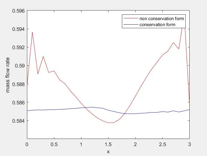
  • Comparison of variation of mass flow rate in both the forms
    • figure(4) plots the variation of mass flow rate through the nozzle at time step 1400 for both non-conservation and conservation form.
    • At this time steps, mass flow rates using both the methods are well converged

    • %comparison of the variation of mass flow rate in both the forms
      figure(4)
      plot(x,m_nc,'r-',x,m_c,'b');
      legend('non conservation form','conservation form');
      xlabel('x')
      ylabel('mass flow rate');

Solution for Non-Conservation form of equations:

equations (1) to (9) expressed above are written in dimensional form but for nozzle flows flow fields are expressed in terms of non-dimensional variables (by taking a ratio of variables with the stagnation values) so rewriting the equation in the non-dimensional form:

Continuity

`(del(rho'))/(delt)=-rho'(del(V'))/(delx')-rho'V'(del(lnA'))/(delx')-V'(delrho')/(delx')`..........................(13)

Momentum

`(delV')/(delt') =-V'(delV')/(delx')-1/gamma((delT')/(delx')+(T')/(rho')(delp')/(delx')`.......................(14)

Energy

`(delT')/(delt')=-V'(delT')/(delx')-(gamma-1)T'[(del(V'))/(delx')-V'(del(lnA'))/(delx')]`......................(15)

equation (13),(14) and (15) needs to be solved using MacCormack's Technique.

code for function:

• initial conditions are defined first as initial profiles in order to obtain the values of primitive variables before begining the time marching, all values at time t is known and the using difference equations values at time t+dt is calculated.
• time loop is initiated for nt number of time steps
• Predictor step: all the spatial derivatives are setup in forward difference for predictor step as follows:
  • `((delrho)/(delt))_i^t=-rho_i^t(V_(i+1)^t-V_i^t)/(Deltax)-rho_i^tV_i^t(lnA_(i+1)-lnA_i)/(Deltax)-V_i^t(rho_(i+1)^t-rho_i^t)/(Deltax)`
  • `((delV)/(delt))_i^t=-V_i^t(V_(i+1)^t-V_i^t)/(Deltax)-1/gamma((T_(i+1)^t-T_i^t)/(Deltax)+T_i^t/rho_i^t(rho_(i+1)^t-rho_i^t)/(Deltax)`
  • `((delT)/(delt))_i^t=-V_i^t(T_(i+1)^t-T_i^t)/(dx)-(gamma-1)T_i^t((V_(i+1)^t-V_i^t)/(dx)-V_i^t(lnA_(i+1)-lnA_i)/(dx))`
  • values of primitive variable are obtained at grid points from 2 to n-1 i.e all except at first and last grid points as they are already calculated.
• Solution update: In this step, we predict the values of primitive variables as follows
  
  • `rho_i^(t+dt)=rho_i^t+((delrho)/(delt))^tDeltat`
  • `V_i^(t+dt)=V_i^t+((delV)/(delt))^tDeltat`
  • `T_i^(t+dt)=T_i^t+((delT)/(delt))^tDeltat`
  • from this step we obtain the values at time t
• Corrector Step:
  • in this step we replace the spatial derivatives by backward differencing as follows:
  • `((delrho)/(delt))_i^(t+Deltat)=-rho_i^(t+Deltat)(V_(i)^(t+Deltat)-V_(i-1)^(t+Deltat))/(Deltax)-rho_i^(t+Deltat)V_i^(t+Deltat)(lnA_(i)-lnA_(i-1))/(Deltax)-V_i^(t+Deltat)(rho_(i)^(t+Deltat)-rho_(i-1)^(t+Deltat))/(Deltax)`
  • `((delV)/(delt))_i^(t+Deltat)=-V_i^(t+Deltat)(V_(i)^(t+Deltat)-V_(i-1)^(t+Deltat))/(Deltax)-1/gamma((T_(i)^(t+Deltat)-T_(i-1)^(t+Deltat))/(Deltax)+T_i^(t+Deltat)/rho_i^(t+Deltat)rho_(i)^(t+Deltat)-rho_(i-1)^(t+Deltat)/(Deltax))`
  • `((delT)/(delt))_i^(t+Deltat)=-V_(i)^(t+Deltat)(T_(i)^(t+Deltat)-T_(i-1)^(t+Deltat))/(Deltax)-(gamma-1)T_i^(t+Deltat)((V_(i)^(t+Deltat)-V_(i-1)^(t+Deltat))/(Deltax)-V_i^(t+Deltat)(lnA_(i)-lnA_(i-1))/(Deltax))`
• Computing the average time derivatives:
  
  • now we calculate the average time derivative from predictor and corrector step
  • `((delrho)/(delt))_(av)=0.5[((delrho)/(delt))_i^t+((delrho)/(delt))_i^(t+Deltat)]`
  • `((delV)/(delt))_(av)=0.5[((delV)/(delt))_i^t+((delV)/(delt))_i^(t+Deltat)]`
  • `((delT)/(delt))_(av)=0.5[((delT)/(delt))_i^t+((delT)/(delt))_i^(t+Deltat)]`
• Updating final solution
  
  • finally using the average values, the final values of flow field variables are obtained at time t+`Deltat` as follows
  • `rho_i^(t+dt)=rho_i^t+((delrho)/(delt))_(av)^tDeltat`
  • `V_i^(t+dt)=V_i^t+((delV)/(delt))_(av)^tDeltat`
  • `T_i^(t+dt)=T_i^t+((delT)/(delt))_(av)^tDeltat`
  • This completes the macCormack's method
• Boundary Conditions:
  • The boundary consists of the inflow boundary, through which the flow coming from the reservoir, enters the nozzle. The second boundary is the outflow boundary where flow leaves the nozzle.
  • In order to find out the inflow and outflow boundary conditions, it is important to have a look at the characteristics and streamlines which can be observed in the figure as follows:
  • 
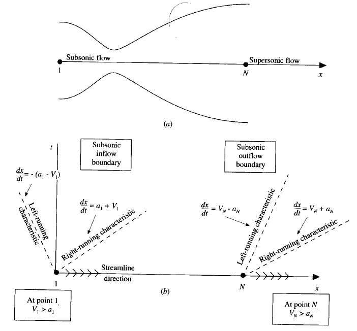
  • According to the method of characteristics, if one characteristic propagates into the domain, then the value of one dependent variable must be specified at that boundary. If another characteristic propagates out of the domain, then the value of one dependent variable must be allowed to float at the boundary. Also if streamline is moving into the domain, the second variable must be specified at the inflow.
  • Thus, at the subsonic inflow boundary, we must specify two dependent variables and one floating variable.
    • floating variable: `V_1=2V_2-V_3`
    • Fixed variables: `rho=1, T=1`
  • Similarly, at the outflow, both the characteristics flow out of the domain and streamline also flow out. hence no variables are specified at the outflow boundary and all variables must be allowed to float.
    
    • `V_n=2V_(n-1)-V_(n-2)`
    • `rho_n=2rho_(n-1)-rho_(n-2)`
    • `T_n=2T_(n-1)-T_(n-2)`
• After this step, we have completed the analysis and calculated the rho, V, and T. The remaining variables (M. mass flow rate and p) are calculated.
• The timewise variations of all variables are at the throat section are stored separately for plotting a result.
• variation of mass flow rates at different time step is plotted in figure 4.

function [rho,v,t,M,p,rho_nc_t,t_nc_t,p_nc_t,M_nc_t,m]=nonc(gamma,dx,nt,dt,n,x,throat);

%initial profiles
rho=1-0.3146*x;
t=1-0.2314*x;
v=(0.1+1.09*x).*t.^0.5;
a=1+2.2*(x-1.5).^2;

for k=1:nt
    rho_old=rho;
    v_old=v;
    t_old=t;
    %predictor method
    for j=2:n-1
        
        dvdx=(v(j+1)-v(j))/dx;
        drhodx=(rho(j+1)-rho(j))/dx;
        dtdx=(t(j+1)-t(j))/dx;
        dlog_a_dx=(log(a(j+1))-log(a(j)))/dx;
        
        %continuity
        drhodt_p(j)=-rho(j).*dvdx-rho(j).*v(j)*dlog_a_dx-v(j).*drhodx;
        
        %momentum equation
        dvdt_p(j) =-v(j).*dvdx-(1/gamma).*(dtdx+(t(j)/rho(j)).*drhodx);
        
        %energy equation
        dtdt_p(j)=-v(j).*dtdx-(gamma-1).*t(j).*(dvdx+(v(j).*dlog_a_dx));
        
        
       %solution update
       rho(j)=rho(j)+drhodt_p(j)*dt;
       v(j)=v(j)+dvdt_p(j)*dt;
       t(j)=t(j)+dtdt_p(j)*dt;
    end
    
    %corrector method
    for j=2:n-1
        
        dvdx=(v(j)-v(j-1))/dx;
        drhodx=(rho(j)-rho(j-1))/dx;
        dtdx=(t(j)-t(j-1))/dx;
        dlog_a_dx=(log(a(j))-log(a(j-1)))/dx;
        
        %continuity
        drhodt_c(j)=-rho(j).*dvdx-rho(j).*v(j)*dlog_a_dx-v(j).*drhodx;
        
        %momentum equation
        dvdt_c(j) =-v(j).*dvdx-(1/gamma).*(dtdx+(t(j)/rho(j)).*drhodx);
        
        %energy equation
        dtdt_c(j)=-v(j).*dtdx-(gamma-1).*t(j).*(dvdx+(v(j).*dlog_a_dx));
    end
        
    %compute average time derivative
    drhodt=0.5*(drhodt_p+drhodt_c);
    dvdt=0.5*(dvdt_p+dvdt_c);
    dtdt=0.5*(dtdt_p+dtdt_c);
       
    %final solution update
    for i=2:n-1
        rho(i)=rho_old(i)+drhodt(i)*dt;
        v(i)=v_old(i)+dvdt(i)*dt;
        t(i)=t_old(i)+dtdt(i)*dt;
    end
    
    %apply boundary conditions
    %inlet
    v(1)=2*v(2)-v(3);
    %outlet
    rho(n)=2*rho(n-1)-rho(n-2);
    v(n)=2*v(n-1)-v(n-2);
    t(n)=2*t(n-1)-t(n-2);
    
 
    %defining othe flow field variables
    M=v./(t.^0.5);
    p=rho.*t;
    m=rho.*a.*v;
    %mass flow rate w.r.t initial conditions
    m_0t=rho_old.*a.*v_old;
    
    %storing values of primitive variables at throat w.r.t to time steps
    rho_nc_t(k)=rho(throat);
    M_nc_t (k)=v(throat)./(t(throat).^0.5);
    p_nc_t (k)=rho(throat).*t(throat);
    t_nc_t(k)=t(throat);
  
%Instantaneous distribution of nondimensional mass flow as a function of distance through the nozzle at five different times during the time marching approach to the steady state 
figure(3)
subplot(2,1,1);
if k==50
    plot(x,m,'b');
    hold on
elseif k==100
    plot(x,m,'r');
elseif k==150
    plot(x,m,'m');
elseif k==200
    plot(x,m,'c');
elseif k==850
    plot(x,m,'g');
end
xlabel('non-dimensional distance through nozzle (x)');
ylabel('non-dimensional mass flow rate');
legend('50','100','150','200','850')  
end

Solution for Conservation form of equations:

Continuity:

`(del rho'A')/(delt')+(del(rho'A'V'))/(delx')=0`....................(10)

Momentum

`(del(rho'V'A'))/(delt') + (del(rho'A'V'^2+(1/gamma)p'A'))/(delx') = -1/gamma p'(delA')/(delx')`.......................(11)

Energy

`(del[rho'((e')/(gamma-1)+gamma/2V'^2)A'])/(delt')+(del[rho'((e')/(gamma-1)+gamma/2V'^2)V'A'+rho'A'V'])/(delx')=0`.............(12)

The nondimensional conservation forms of equation can be expressed in generic form for quasi-one dimensional flows

`(delU)/(delt)+(delF)/(delx)=J`

U= solution vector, F=Flux vector and J=source term

for above equations U,F and J are defined as follows,

`U_1=rho'A'`

`U_2=rho'A'V'`

`U_3=rho'((e')/(gamma-1)+gamma/2V'^2)A'`

`F_1=rho'A'V'=U_2`

`F_2=rho'A'V'+1/gammap'A'=(U_2^2)/(U_1)+(gamma-1)/(gamma)(U_3-gamma/2(U_2^2)/(U_1))`

`F_3=rho'((e')/(gamma-1)+gamma/2V'^2)V'A'+p'A'V'=gamma(U_2U_3)/(U_1)-(gamma(gamma-1))/(2)(U_2^3)/(U_1^2)`

`J_2=1/gammap'(delA')/(delx')=(gamma-1)/(gamma)(U_3-gamma/2(U_2^2)/(U_1))(dellnA')/(delx')`

using the expressions equations can be written to represent continuity, momentum and energy equation respectively as follows

`(delU_1)/(delt')=-(delF_1)/(delx')`................(13)

`(delU_2)/(delt')=-(delF_2)/(delx')+J_2`............(14)

`(delU_3)/(delt')=-(delF_3)/(delx')`...............(15)

equations (13),(14) and (15) are the pure forms of governing equations in conservation form that will be used to solve the system using MacCormack's Technique.

when the coding of the solution of govening equations is done using the pure form, the solution is stable and converges to a steady state is achieved. It is observed that implementing F1,F2,F3, and J2 is terms of primitive variables could lead to instabilities in the solution hence expressions in terms of U1,U2 and U3 are used.

code for function:

• Since the sensitivity of numerical computation is more sensitive, improved initial conditions for rho and T are defined. the initial profiles are used to obtain the values of primitive variables before beginning the time marching. once all values at time t are known then using difference equations values at time t+dt are calculated.
• Then the initial conditions of V, U1, U2, and U3 are defined.
• the time loop is initiated for nt number of time steps
• Predictor step: all the spatial derivatives are setup in forward difference for the predictor step as follows:
  • `((delU_1)/(delt'))_i^(t)=-((F_1)_(i+1)-(F_1)_(i))/(Deltax)`
  • `((delU_2)/(delt'))_i^(t)=-((F_2)_(i+1)-(F_2)_(i))/(Deltax)+J_2`
  • `((delU_3)/(delt'))_i^(t)=-((F_3)_(i+1)-(F_3)_(i))/(Deltax)`
  • values of the pure variables are obtained at grid points from 2 to n-1 i.e all except at first and last grid points as they are already calculated.
• Solution update: In this step, we predict the values of primitive variables as follows
  
  • `(U_1)_i^(t)=(U_1)_i^t+((delU_1)/(delt))^tDeltat`
  • `(U_2)_i^(t)=(U_2)_i^t+((delU_2)/(delt))^tDeltat`
  • `(U_3)_i^(t)=(U_3)_i^t+((delU_3)/(delt))^tDeltat`
  • from this step we obtain the values at time t
• Corrector Step:
  • in this step we replace the spatial derivatives by backward differencing as follows:
  • `((delU_1)/(delt))_i^(t+Deltat)=-((F_1)_(i)-(F_1)_(i-1))/(Deltax)`
  • `((delU_2)/(delt))_i^(t+Deltat)=-((F_2)_(i)-(F_1)_(i-1))/(Deltax)+J_2`
  • `((delU_3)/(delt))_i^(t+Deltat)=-((F_3)_(i)-(F_3)_(i-1))/(Deltax)`
• Computing the average time derivatives:
  
  • now we calculate the average time derivative from predictor and corrector step
  • `((delU_1)/(delt))_(av)=0.5[((delU_1)/(delt))_i^t+((delU_1)/(delt))_i^(t+Deltat)]`
  • `((delU_2)/(delt))_(av)=0.5[((delU_2)/(delt))_i^t+((del(U_2))/(delt))_i^(t+Deltat)]`
  • `((delU_3)/(delt))_(av)=0.5[((delU_3)/(delt))_i^t+((delU_3)/(delt))_i^(t+Deltat)]`
• Updating final solution
  
  • finally using the average values, the final values of flow field variables are obtained at time t+`Deltat` as follows
  • `(U_1)_i^(t+dt)=(U_1)_i^t+((delU_1)/(delt))_(av)^tDeltat`
  • `(U_2)_i^(t+dt)=(U_2)_i^t+((delU_2)/(delt))_(av)^tDeltat`
  • `(U_3)_i^(t+dt)=(U_3)_i^t+((delU_3)/(delt))_(av)^tDeltat`
  • Calculate the primitive variables from basic definitions of U1,U2 and U3.
• Boundary Conditions:
  • The boundary conditions hold a similar explanation as in the case of non-conservation form
  • thus, for inflow boundary, by keeping rho and t fixed and floating v the boundary conditions are obtained as follows:
    • `U_(1(i=1))=A_(1(i=1))=fixed`
    • `U_(2(i=1))=2U_(2(i=2))-U_(2(i=3))`
    • `U_((i=1))=U_(1(i=1))((T')/(gamma-1)+(gamma)/2V_(1(i=1))'^2)`
  • Similarly, the outflow boundary conditions are as follows
    
    • `(U_1)_n=2(U_1)_(n-1)-(U_1)_(n-2)`
    • `(U_1)_n=2(U_1)_(n-1)-(U_1)_(n-2)`
    • `(U_1)_n=2(U_1)_(n-1)-(U_1)_(n-2)`
• After this step, we have completed the analysis and calculated the rho, V, and T. The remaining variables (M. mass flow rate and p) are calculated.
• The timewise variations of all variables are at the throat section are stored separately for plotting a result.
• variation of mass flow rates at different time steps is plotted in figure 4.

function [rho,v,t,p,M,rho_c_t,t_c_t,p_c_t,M_c_t,m]=conv(gamma,dx,x,n,nt,dt,throat);

%initial profiles
for i=1:n
    if (x(i)<0.5)
        rho(i)=1;
        t(i)=1;
    elseif (x(i)>=0.5 && (x(i)<=1.5))
        rho(i)=1-(0.366*(x(i)-0.5));
        t(i)=1-(0.167*(x(i)-0.5));
    else
        rho(i)=0.634-(0.3879*(x(i)-1.5));
        t(i)=0.833-(0.3507*(x(i)-1.5));
    end
end

a=1+2.2*(x-1.5).^2;
v=0.59./(rho.*a);
u1=rho.*a;
u2=rho.*a.*v;
u3=u1.*((t./(gamma-1))+((gamma/2).*(v.^2)));
    
for k=1:nt
    u1_old=u1; %i=31 only copies the last element of u1,u2 and u3
    u2_old=u2;
    u3_old=u3;
    
    %flux 
    f1=u2;
    f2=((u2.^2)./u1)+(((gamma-1)/gamma).*(u3-((gamma/2)*((u2.^2)./u1))));
    f3=(((gamma.*u2.*u3)./u1)-(gamma.*((gamma-1)/2).*((u2.^3)./(u1.^2))));
    
    %predictor step
    for j=2:n-1
      
     du1dt_p(j)=-(f1(j+1)-f1(j))/dx;
     j2(j)=(1/gamma)*rho(j)*t(j)*((a(j+1)-a(j))/dx);
     du2dt_p(j)=-(f2(j+1)-f2(j))/dx+j2(j);
     du3dt_p(j)=-(f3(j+1)-f3(j))/dx;
     
     %solution update
     u1(j)=u1(j)+du1dt_p(j)*dt;
     u2(j)=u2(j)+du2dt_p(j)*dt;
     u3(j)=u3(j)+du3dt_p(j)*dt;

  end
    %primitive variables update
     rho=u1./a;
     v=u2./u1;
     t=(gamma-1).*((u3./u1)-((gamma/2).*(v.^2)));
    %flux update for corrector
    f1=u2;
    f2=((u2.^2)./u1)+(((gamma-1)/gamma).*(u3-((gamma/2)*((u2.^2)./u1))));
    f3=(((gamma.*u2.*u3)./u1)-(gamma.*((gamma-1)/2).*((u2.^3)./(u1.^2))));
     
     
    %corrector method
    for j=2:n-1
        
        df1dx=((f1(j)-f1(j-1))/dx);
        df2dx=((f2(j)-f2(j-1))/dx);
        df3dx=((f3(j)-f3(j-1))/dx);
        
        %continuity
        du1dt_c(j)=-df1dx;
        j2(j)=(1/gamma)*rho(j)*t(j)*((a(j)-a(j-1))/dx); %j2 has to be recalculated with backward difference
        %momentum equation
        du2dt_c(j)=-df2dx+j2(j);
        
        %energy equation
        du3dt_c(j)=-df3dx; %No j2 for du3dt
    end
        
    %compute average time derivative
    du1dt=0.5*(du1dt_p+du1dt_c);
    du2dt=0.5*(du2dt_p+du2dt_c);
    du3dt=0.5*(du3dt_p+du3dt_c);
       
    %final solution 
    for i=2:n-1
        u1(i)=u1_old(i)+du1dt(i)*dt;
        u2(i)=u2_old(i)+du2dt(i)*dt;
        u3(i)=u3_old(i)+du3dt(i)*dt;
    end
    %apply boundary conditions
    %inlet
    u2(1)=2*u2(2)-u2(3);
    v(1)=u2(1)/u1(1);
    u3(1)=u1(1)*((t(1)/(gamma-1))+(0.5*gamma*v(1)^2));
    %outlet
    u1(n)=2*u1(n-1)-u1(n-2);
    u2(n)=2*u2(n-1)-u2(n-2);
    u3(n)=2*u3(n-1)-u3(n-2);
    
     %Final primitive variables update 
     rho=u1./a;
     v=u2./u1;
     t=(gamma-1).*((u3./u1)-((gamma/2).*(v.^2)));
     
   %defining othe flow field variables
    M=v./(t.^0.5);
    p=rho.*t;
    m=rho.*a.*v;
    
    %storing values of primitive variables at throat w.r.t to time steps
    rho_c_t(k)=rho(throat);
    t_c_t(k)=t(throat);
    p_c_t(k)=rho(throat);
    M_c_t(k)=M(throat);
    
%Instantaneous distribution of nondimensional mass flow as a function of distance through the nozzle at five different times during the time marching approach to the steady state     
figure(3)
subplot(2,1,2);
if k==50
    plot(x,m,'b');
    hold on
elseif k==100
    plot(x,m,'r');
elseif k==150
    plot(x,m,'m');
elseif k==200
    plot(x,m,'c');
elseif k==800
    plot(x,m,'g');
end    
xlabel('non-dimensional distance through nozzle (x)');
ylabel('non-dimensional mass flow rate');
legend('50','100','150','200','800')
end

Results:

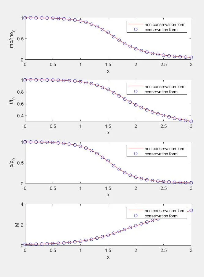
Figure 1:Steady-state distribution of primitive variables inside the nozzle

• The figure represents the steady-state variation of primitive variables along the length x for both conservation and non-conservation forms.
• The variables computed from both the methods show exact same variations
• The density, temperature, and pressure decrease as the flow proceeds along the length of the nozzle.
• The Mach no. is <1 (subsonic) at nozzle entry, =1 at throat and >1 (supersonic) at nozzle exit.

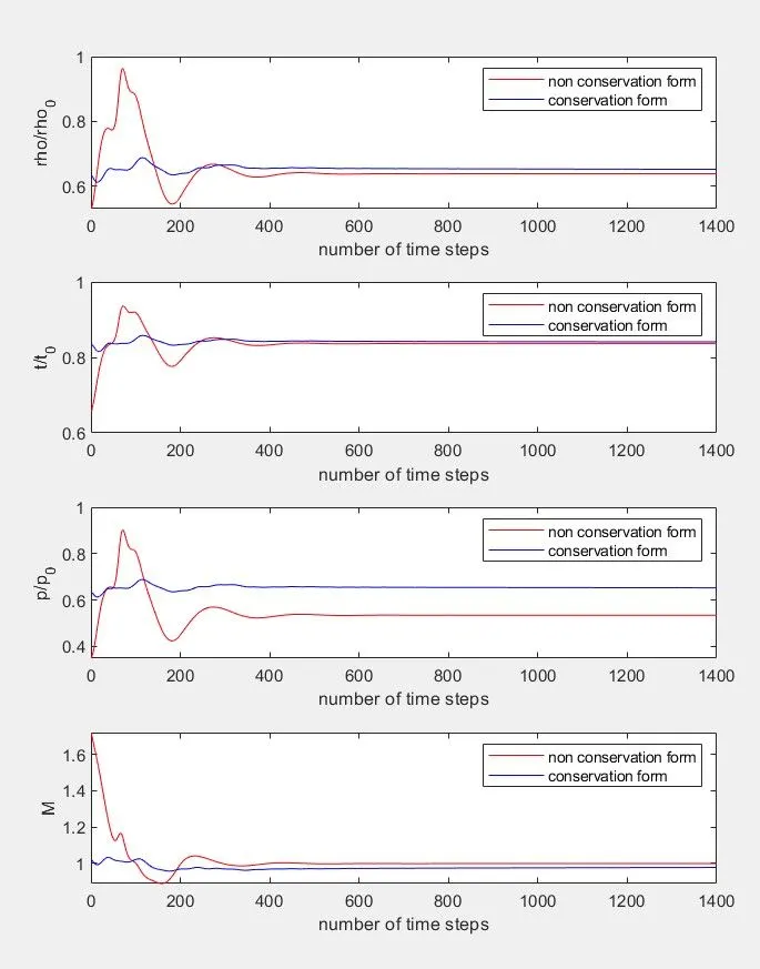
Figure(2): Time-wise variation of the primitive variables

• The figure demonstrates the timewise variation of the primitive variables with respect to the number of time steps for both conservation and non-conservation forms.
• It is observed that the variations are large at smaller time steps, the changes in the flow field variables reduce at a larger value of time steps when the solution approaches a steady state.
• It can also be observed that initial variations in the case of conservation form are much lesser compared to that of non-conservation form which is probably due to a more improved definition of the initial condition in the case of the former.

Figure(3) Variation of Mass flow rate distribution inside the nozzle at different time steps during the time-marching process

• The figure demonstrates the variation of the mass flow rate along the length of the nozzle at different time steps for both conservation and non-conservation forms.
• The different curves represent a variation of mass flow after 50,100, 150, 200, and 850-time steps for the non-conservation form, and the last timestep for conservation form is 800.
• It is observed the variation changes drastically after these time steps, slowly approaching towards a constant value at the 850th time step in case of non-conservation form and at 8000 at conservation form. This indicates that the mass flow rate is converged to a constant, steady-state value throughout the nozzle.

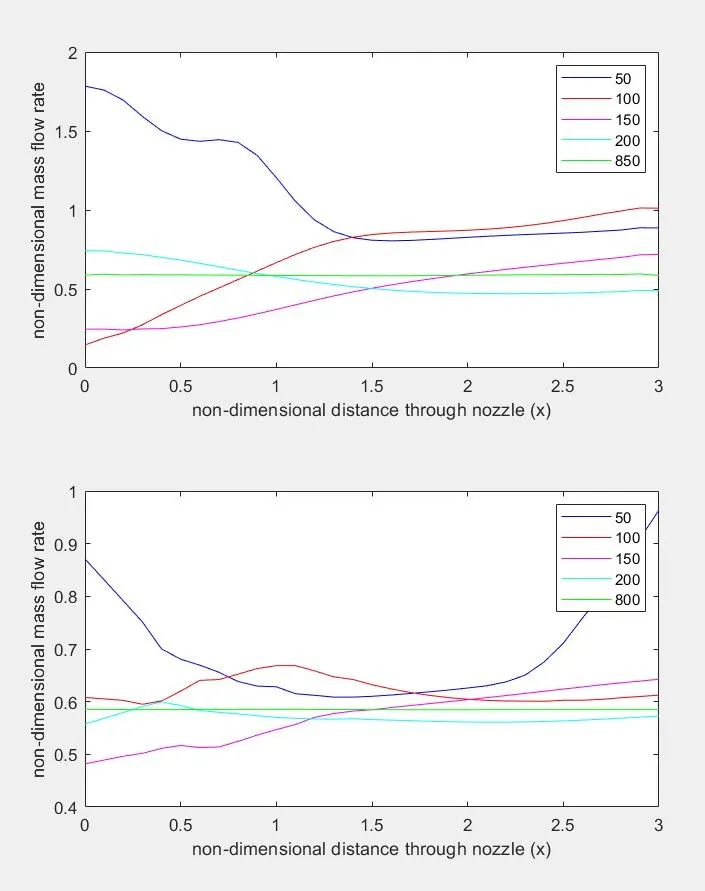
Figure (4) Comparison of Normalized mass flow rate distributions of Non-conservation and Conservation form

• The figure represents a comparison of the normalized mass flow rate distribution between both forms.
• The comparison suggests that the conservation form preserves the mass flow rate throughout the flow field in a better manner than the nonconservation form.
• This is because the mass flow rate is a primary result of these equations (U2=rho*A*V). while in case of non-conservation form the mass flow rate is obtained as a secondary result
• As the conservation form does a better job of conserving the mass flow rate we can understand why they are called conservation form.

Conclusion:

• The non-conservation forms of equations can be implemented directly in non-dimensional forms while in the case of conservation form non-dimensional equations must be represented in pure forms to obtain a stable solution.
• The numerical solution using the conservation form is more sensitive and thus requires improved definitions of initial conditions and implementation in the pure form of governing equations.