Week 5.1 - Mid term project - Solving the steady and unsteady 2D heat conduction problem

Theory of solution of a system of equations: Direct and Iterative Solvers

• Once we perform discretization we are left with the system of equation. These systems of equations can be solved using the following two methods: 1. Direct method 2.Iterative solvers.
• Cramer's rule and the gauss elimination method are popular examples of direct methods. In the direct method, we can identify the number of iterations in advance. Iterative methods are based on solving simple algorithms repeatedly till the solution reaches convergence. In iterative solvers, it is not possible to predict the number of iterations in advance. The direct methods require more memory as compared to iterative solvers (as only non-zero coefficients of the equations are required to be stored in memory). Thus, iterative methods become more economical compared to the direct methods for applications of CFD (as CFD problems can be very large).
• The Jacobi and Gauss-Siedel method are examples of Point Iterative Solvers. These methods are easy to implement but they can have slower convergence rates in case of a large system of equations. However, their convergence rate can be improved with the help of multigrid accelerators.
• To understand the solution of a system of equations using iterative solvers, consider the following example:
  • Consider the system of equations:
    • T1+2*T2+3*T3=0
    • -T1+5*T2-6*T3=0
    • 7*T1+8*T2-0.5*T3=0
  • we first take initial guesses for values T1, T2 and T3. using these values we can calculate the unknowns. These values are then calculated iteratively till the solution converges. The difference between the Jacobi and Gauss Siedel is the substitution it makes:
    • The substitution for Jacobi Method in the matrix form is as follows:
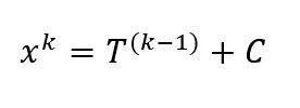      • where T is the iteration matric and C is the constant vector.
    • The substitution for Gauss-Siedel Method in the matrix form is as follows:
      • where T is the iteration matric and C is the constant vector.

Relaxation Methods :

• The properties of the convergence matrix affect the rate of convergence for Jacobi and Gauss-Siedel methods. These properties can be improved with the introduction of a relaxation parameter w.
• if the value of w lies between 0 and 1 the method is called the under-relaxation method and if w>1 it is called over-relaxation.
• The use optimum value of the relaxation factor minimizes the number of iterations required to reach the converged solution. however, finding the optimum value of the relaxation parameter is not easy and can be predicted with experience.
• In the current problem Successive Over Relaxation (SOR) technique is applied to the Gauss-Siedel method.

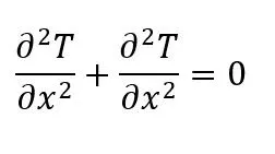
Steady-State 2D Heat Conduction

• `
  • as the term in the steady-state heat conduction equation is elliptical in nature we need to take information from all directions, thus we use the central differencing scheme.
  • 
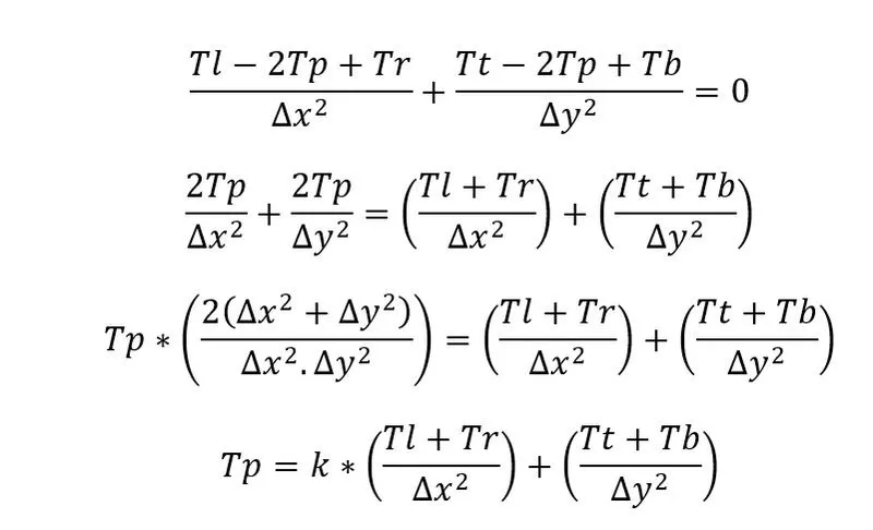
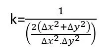
  • where k is given by
  • 
• Applying boundary conditions:
  
  • To initial and boundary conditions:
    
    • We first generate a matrix (nx x ny) and assign it with initial conditions of say T=300K
    • T=300*ones(nx,ny) generates a matrix (nx X ny) so that value of all the elements of this matrix is equal to 300K
    • In order to update the matrix with the boundary conditions we call elements of the matrix and assign different values to these elements
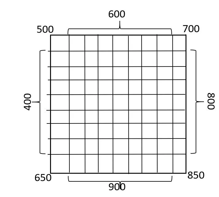
      • for eg: T(1,2:(ny-1)=600 updates the values of 1st row and columns 2 to ny-1 to 600. After definition of all the boundary conditions the matrix would look as shown in the 1st figure
• After defining the boundary conditions the grid should look as follows :
  • 

  • clear all
    close all
    clc
    
    %input
    nx=10;
    ny=nx;
    T=300*ones(nx,ny);
    
    %applying boundary conditions
    T(1,2:(ny-1))=600;
    T(2:(nx-1),1)=400;
    T(nx,2:(ny-1))=900;
    T(2:(nx-1),ny)=800;
    T(1,1)=500;
    T(1,ny)=700;
    T(nx,ny)=850;
    T(nx,1)=650;

• Generating the grid:
  • The x and y vectors are defined using linspace command.
  • The dx and dy is defined
  • Meshgrid command is used to generate a grid. Meshgrid transforms the domain which is specified by the vectors x and y into arrays X and Y.

  • %generating the grid
    x=linspace(0,1,nx);
    dx=x(2)-x(1);
    y=linspace(0,1,ny);
    dy=y(2)-y(1);
    
    [X,Y]=meshgrid(x,y);

• all the remaining parameters can be defined now. it is important that Told=T is defined after applying the boundary conditions otherwise it won't be updated with these values.
  • error specified here is a random value assigned to initial the convergence loop. it is essential that the value for error is greater than the tolerance.
  • w is the relaxation factor useful while implementing SOR. value of w must be >1. if the value of w is equal to 1.9,2, etc the solution does not converge this is due to the fact that the solution oscillates and does not reach desired.
  • Thus for this problem w=1.1,1.2.

  • Told=T;
    
    iterative_solver=3
    error=9e9;
    tol=1e-4;
    w=1.2;

• Defining the convergence loop for Jacobi solver:
  • we first assign a number to the Jacobi solver as iterative solver=1 and the code initiates the Jacobi solver loop only when the iterative solver is equal to 1.
  • The Jacobi iter term is defined to calculate the number of iterations once the solution converges.
  • next, we initiate a while loop so that the loop continues till the error value > tolerance
  • in the next step we initiate the space loop for in x and y-direction. we start the loop for 2:nx-1 since we already know the Temperature at 1 and nx (boundary condition.
  • Substitution is made T(i,j) as follows,
    • 
    • The error is computed as the maximum of the difference of absolute of Told-T.
    • The Told is updated to T computed from the loop. it is important to define Told=T after the error values as if defined prior the error will always be zero and the loop will not execute.
    • In the next step, the Jacobi iter is updated.
  • plotting the contour plot
    • Lastly, we plot a contour plot for the given solution. a contour matrix [M, N] is defined using contourf command. contourf helps create a filled contour plot containing the isolines of matrix x,y.
    • The clabel command labels the current contour plot with rotated text inserted into each contour line.
    • The colormap(jet) command sets the colormap of the figure to a selection of colors from the jet color scheme.
    • colorbar command displays a bar to indicate the mapping of data values into the colormap.
    • The title of the text is updated for each value of Jacobi iteration with the help of sprintf command which formats data into string or character vector

  • if iterative_solver==1
        jacobi_iter=1
        while(error>tol)
            for i=2:nx-1
                for j=2:ny-1
                    k=(2*(((dx^2)+(dy^2))/((dx^2)*(dy^2))))^(-1);
                    T(i,j)=k*(((Told(i-1,j)+Told(i+1,j))/(dx^2))+((Told(i,j-1)+Told(i,j+1))/(dy^2)));
                end
            end
            error=max(max(abs(Told-T)));
            Told=T;
            jacobi_iter=jacobi_iter+1;
            
            %plotting
            [M, N]=contourf(X,Y,flipud(T))
            clabel(M,N)
            colormap(jet)
            colorbar
            title_text=sprintf('jacobi steady state number of iterations = %d',jacobi_iter)
            title(title_text);
            xlabel('x axis')
            ylabel('Y axis')
            pause(0.03)
        end
    end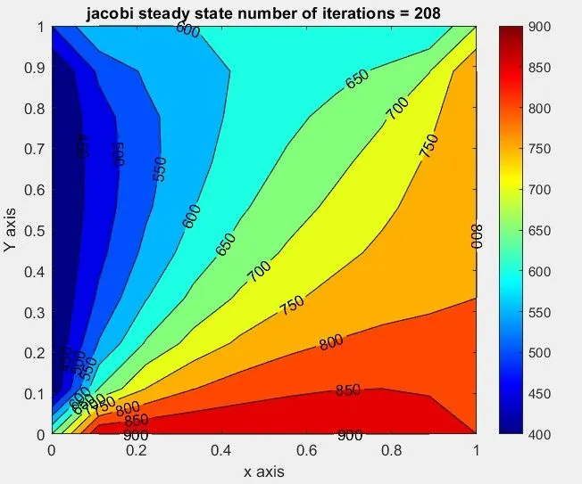

  • 
  • From the figure, we can see that we require 208 iterations to get the desired solution to the 2D steady-state heat conduction equation using the Jacobi method.

• Defining the convergence loop for Gauss-Siedel solver:
  • we first assign a number to the Gauss-Siedel solver as iterative solver=2 and the code initiates the GS solver loop only when the iterative solver is equal to 2.
  • Substitution is made T(i,j) as follows,
    • 

  • if iterative_solver==2
        gs_iter=1
        while(error>tol)
            for i=2:nx-1
                for j=2:ny-1
                    k=(2*(((dx^2)+(dy^2))/((dx^2)*(dy^2))))^(-1);
                    T(i,j)=k*(((T(i-1,j)+T(i+1,j))/(dx^2))+((T(i,j-1)+T(i,j+1))/(dy^2)));
                end
            end
            error=max(max(abs(Told-T)));
            Told=T;
            gs_iter=gs_iter+1;
            
            %plotting
            [M, N]=contourf(X,Y,T)
            clabel(M,N)
            colormap(jet)
            colorbar
            title_text=sprintf('Gauss-Seidel steady state number of iterations = %d',gs_iter)
            title(title_text);
            xlabel('x axis')
            ylabel('Y axis')
            pause(0.03)
        end
    end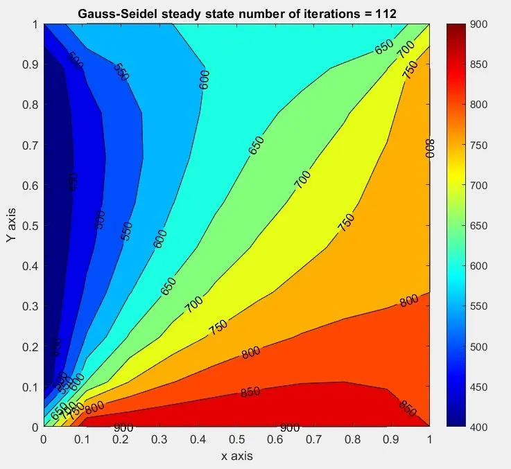

  • 
  • From the figure, we can see that we require 112 iterations to get the desired solution to the 2D steady-state heat conduction equation using the GS method.

• Defining the convergence loop for Successive Over Relaxation :
  • we first assign a number to the SOR solver as iterative solver=3 and the code initiates the SOR solver loop only when the iterative solver is equal to 3.
  • Substitution is made T(i,j) as follows,
  • 
  • where the value of w for the current problem is taken as 1.2.
  
  

  • if iterative_solver==3
        SOR_iter=1
        while(error>tol)
            for i=2:nx-1
                for j=2:ny-1
                    k=(2*(((dx^2)+(dy^2))/((dx^2)*(dy^2))))^(-1);
                    T(i,j)=(1-w)*Told(i,j)+w*(k*(((T(i-1,j)+T(i+1,j))/(dx^2))+((T(i,j-1)+T(i,j+1))/(dy^2))));
                end
            end
            error=max(max(abs(Told-T)));
            Told=T;
            SOR_iter=SOR_iter+1;
            
            %plotting
            [M, N]=contourf(X,Y,T)
            clabel(M,N)
            colormap(jet)
            colorbar
            title_text=sprintf('SOR steady state number of iterations = %d',SOR_iter)
            title(title_text);
            xlabel('x axis')
            ylabel('Y axis')
            pause(0.03)
        end
    end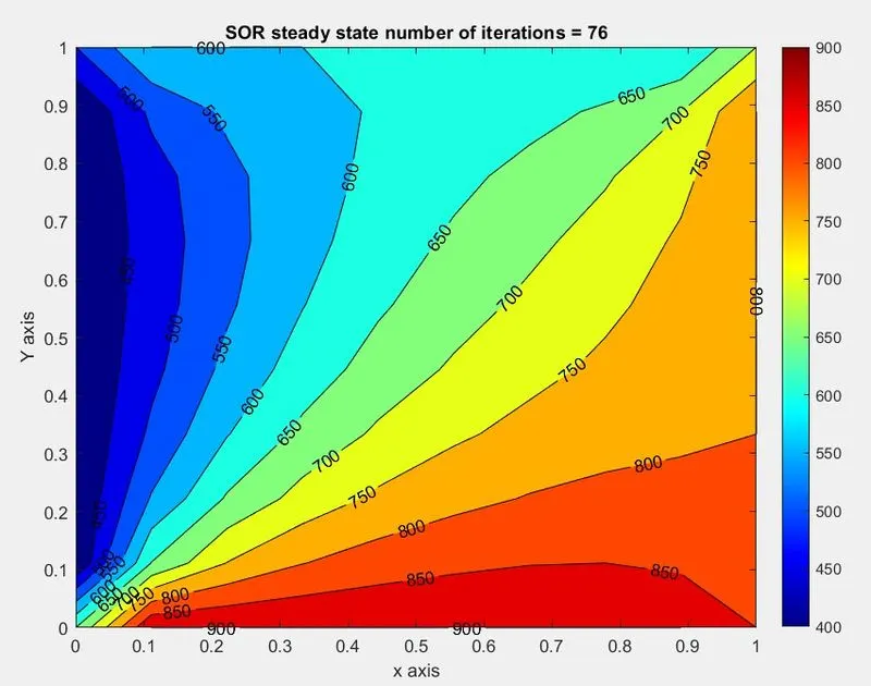

  • 
  • From the figure, we can see that we require 76 iterations to get the desired solution to the 2D steady-state heat conduction equation using the SOR method.

• Conclusion:
  
  • from the above solution, we conclude that the number of iterations for the Jacobi, GS, and SOR method comes out to be 208,112, and 76 respectively.
  • The effect of relaxation methods in increasing the rate of converges of the GS method so that the solution converges faster can be seen as the number of iterations reduce from 112 without relaxation to 76 with relaxation.

Transient 2D Heat Conduction

Theory of Explicit and Implicit Solvers:

Explicit Solver:

• In the explicit method, the value of the parameter to be computed (eg. T in this case) is known at all grid points at time level n (because of the boundary conditions and initial conditions defined). There exists only one unknown T at n+1 whose value is computed using the known values of T at all grid points at time n. As there is a single equation and single unknown it is very is to compute the solution.
• Advantage: Simple in application
• Disadvantage: The time step size (dt) is limited by the stability criteria (CFL number due to the problem of diffusion occurring in this case). the dt is generally very small and may result in larger computational time for a solution.

Implicit Solver:

• In the implicit method, the value of the parameter to be computed (eg. T in this case) is known at all grid points at time level n (because of the boundary conditions and initial conditions defined). While computing the value of T at n+1 we require information from one point at time step n as well as time step n+1. Thus, it will result in x number of equations for x number of unknowns i.e a system of equations.
• The system of equations can be solved directly but this method is not feasible in the case of large systems. Thus, for such a case, we use the iterative solvers to obtain the solution.
• Advantage: No stability restricitions on dt and large values of dt can be used thus, reducing computational time.
• Disadvantages: Difficult to set up a problem.

Transient 2D Heat Conduction (Explicit)

• All the input parameters and boundary conditions applied in a similar way as in the steady-state case. The additional parameter defined is dt=0.001 and alpha=1.4, as shown below.
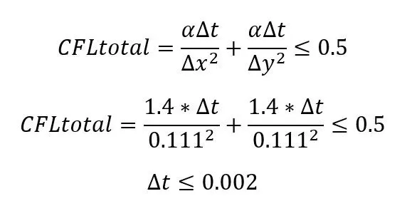
• In Explicit Solver, Diffusion problem occurs therefore total CFL (CFLx+CFLy) must be < 0.5.
• Iterative solvers are not required to solve the problem using an explicit method.
• The first is the time loop which is defined to run for 200-time steps.
• In the next step, we initiate the space loop for in x and y-direction. we start the loop for 2:nx-1 since we already know the Temperature at 1 and nx (boundary condition).
• Substitution is made T(i,j) as follows,
  • 
  • where,
  • 
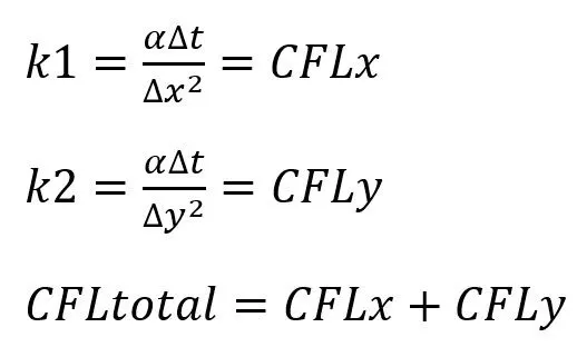
  • The value of dt is limited by CFL to be <0.002 as shown below,
  • 
  • In the case of the explicit method the value of Temperatures at all locations is computed at time t=2 and then the time loop increments by one and at time t=3 again all the values of Temperatures is calculated and the process thus continues for 200 time steps. This is also called time marching.
  • The Told is updated to T within the time loop.
  • tic toc command is implemented to calculate the time required to perform the simulation.
  • Finally, the Countour Plot is plotted

  • clear all
    close all
    clc
    
    %input
    nx=10;
    ny=nx;
    alpha=1.4;
    T=300*ones(nx,ny);
    
    %applying boundary conditions
    T(1,2:(ny-1))=600;
    T(2:(nx-1),1)=400;
    T(nx,2:(ny-1))=900;
    T(2:(nx-1),ny)=800;
    T(1,1)=500;
    T(1,ny)=700;
    T(nx,ny)=850;
    T(nx,1)=650;
    
    %generating the grid
    x=linspace(0,1,nx);
    dx=x(2)-x(1);
    y=linspace(0,1,ny);
    dy=y(2)-y(1);
    dt=0.001;
    
    Told=T;
    
    [X,Y]=meshgrid(x,y);
    % Time loop
    tic  
    for nt=1:1400
          %spatial Loop   
          for i=2:nx-1
                for j=2:ny-1
                    k1=(alpha*dt)/(dx^2);
                    k2=(alpha*dt)/(dy^2);
                    T(i,j)=Told(i,j)+(k1*(Told(i-1,j)-2*Told(i,j)+Told(i+1,j)))+(k2*(Told(i,j-1)-2*Told(i,j)+Told(i,j+1)))
                end
            end
            Told=T;
            %plotting
            [M, N]=contourf(X,Y,flipud(T));
            clabel(M,N)
            colormap(jet)
            colorbar
            title('Explicit Transient')
            xlabel('x axis')
            ylabel('Y axis')
    end
    toc
    time=toc
      

• Results:
  • 
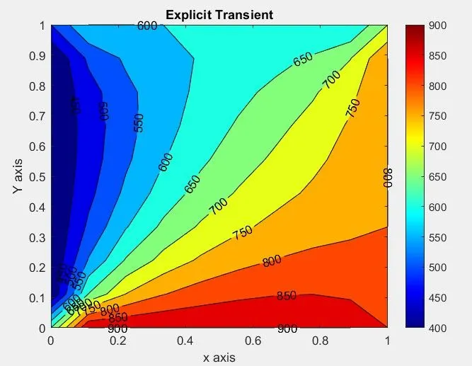
  • We can see the desired result is computed at each time step and the problem is successfully solved using an explicit method.
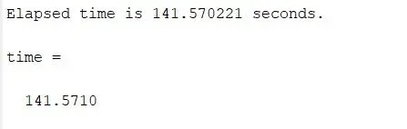
  • Also, the time required to perform the simulation is 141.570 seconds

Transient 2D Heat Conduction (Implicit)

• All the input parameters and boundary conditions applied along with grid generation is performed in a similar way as in the steady-state case. The additional parameters defined are, Tprev=T; dt=1, as shown below.
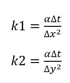
• The constants k1 and k2 are defined as follows:
  • 

• clear all
  close all
  clc
  
  %input
  nx=10;
  ny=nx;
  T=300*ones(nx,ny);
  
  %applying boundary conditions
  T(1,2:(ny-1))=600;
  T(2:(nx-1),1)=400;
  T(nx,2:(ny-1))=900;
  T(2:(nx-1),ny)=800;
  T(1,1)=500;
  T(1,ny)=700;
  T(nx,ny)=850;
  T(nx,1)=650;
  
  %generating the grid
  x=linspace(0,1,nx);
  dx=x(2)-x(1);
  y=linspace(0,1,ny);
  dy=y(2)-y(1);
  
  
  Tprev=T;
  Told=T;
  
  iterative_solver=2;
  error=9e9;
  tol=1e-4;
  w=1.2;
  alpha=2;
  dt=1;
  k1=(alpha*dt)/(dx^2);
  k2=(alpha*dt)/(dy^2);

• Defining the Jacobi solver for transient implicit Method:
  • we first assign a number to the Jacobi solver as iterative solver=1 and the code initiates the Jacobi solver loop only when the iterative solver is equal to 1.
  • The Jacobi iter term is defined to calculate the number of iterations once the solution converges.
  • The time loop is then defined to solve the problem for 1400 time steps.
  • The error value is defined before the while loop so as to forcefully reinitiate this convergence loop f the next time step.
  • next, we initiate a while loop so that the loop continues till the error value > tolerance
  • in the next step we initiate the space loop for in x and y-direction. we start the loop for 2:nx-1 since we already know the Temperature at 1 and nx (boundary condition.
  • Substitution is made T(i,j) as follows,
    • 
    • The error is computed as the maximum of the difference of absolute of Told-T.
    • The Told is updated to T computed from the loop. it is important to define Told=T after the error values as if defined prior the error will always be zero and the loop will not execute.
    • In the next step, the Jacobi iter must be updated inside the time loop to count the convergence iterations.
    • note that the Tprev remains constant till convergence is obtained for one particular time step. it thus must be updated only after the convergence loop within the time loop.
    • tic toc command is implemented to caculate the time required for simulation.
    • finally, the Countour Plot is plotted.

    • %Jacobi_solver
      if iterative_solver==1
          jacobi_iter=1
          tic
          for nt=1:1400
              error = 9e9;
              while error>tol
                  for i=2:nx-1
                      for j=2:ny-1
                          term1=(1+(2*k1)+(2*k2))^(-1);
                          term2=k1*term1;
                          term3=k2*term1;
                          H=Told(i-1,j)+Told(i+1,j);
                          V=Told(i,j-1)+Told(i,j+1);
                          T(i,j)=term1*Tprev(i,j)+term2*H+term3*V;
                      end
                  end
                  error=max(max(abs(Told-T)));
                  jacobi_iter=jacobi_iter+1;
                  Told=T;
              end
              Tprev=T;
              toc
          end
          time=toc;
          
          %plotting
          figure(1)
          [M, N]=contourf(X,Y,flipud(T));
          clabel(M,N)
          colormap(jet)
          colorbar
          title_text=sprintf('jacobi transient implicit number of iterations = %d',jacobi_iter);
          title(title_text);
          xlabel('x axis')
          ylabel('Y axis')
      end

  • Results:
  • 
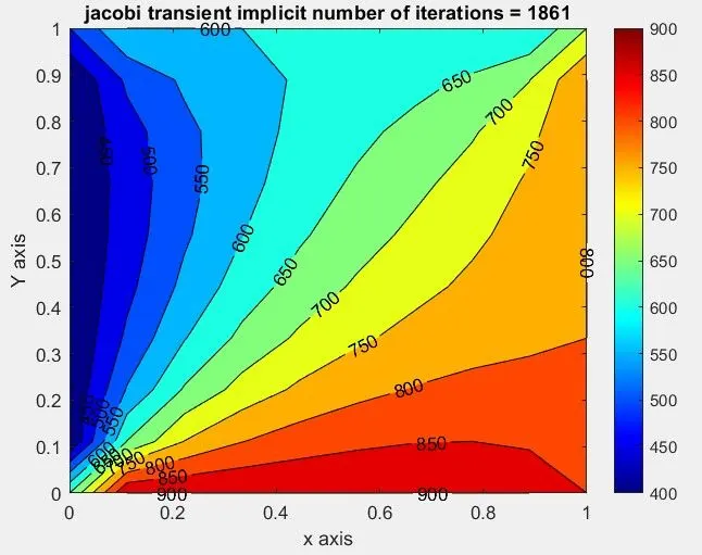
  • From the figure, we can see that we require 1861 iterations to get the desired solution to the 2D transient heat conduction equation using the implicit method and the Jacobi iterative solver.
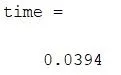
  • Also, the time required to perform the simulation is 0.0394 seconds
  • 

Defining the GS solver for transient implicit Method:

• we first assign a number to the Gauss-Siedel solver as iterative solver=2 and the code initiates the GS solver loop only when the iterative solver is equal to 2.
• Substitution is made T(i,j) as follows,
  • 
• all the remaining process is same as that for Jacobi solver.
• Result:
  • 
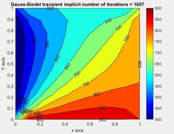
  • From the figure, we can see that we require 1657 iterations to get the desired solution to the 2D transient heat conduction equation using the implicit method and the Gauss-Siedel iterative solver.
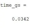
  • Also, the time required to perform the simulation is 0.0342 seconds
  • 
• Defining the Successive Over Relaxation solver for transient implicit Method: :
  • we first assign a number to the SOR solver as iterative solver=3 and the code initiates the SOR solver loop only when the iterative solver is equal to 3.
  • Substitution is made T(i,j) as follows,
  • 
  • where the value of w for the current problem is taken as 1.2.
  • The remaining procedure is the same as that of the Jacobi Solver.
  • Result:
    • 
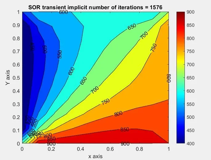
    • From the figure, we can see that we require 1576 iterations to get the desired solution to the 2D transient heat conduction equation using the implicit method and the Successive Over Relaxation over Gauss Siedel iterative solver.
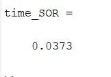
    • Also, the time required to perform the simulation is 0.0373 seconds
    • 

Conclusion:

• To solve the 2D heat conduction problem for Transient simulation using the Explicit method iterative solvers are not required.
• The time required for solving the Explicit method (141) is much greater than the Implicit solver (0.03) as explained in theory, due to the very small value of dt(=0.001) in case of explicit as compared to implicit (dt=1).
• In the case of the solution of the problem using the Implicit Method, we found that the number of iterations are far more than that for steady-state.
  • number of iterations is maximum for Jacobi Method (1861), followed by Gauss-Siedel Method (1657)
  • It can also be observed that the number of iterations can be further reduced by using Successive over relaxation on the Gauss Siedel solver. The number of iterations for this case is the least (1576).