Week 3.5 - Deriving 4th order approximation of a 2nd order derivative using Taylor Table method
- central differencing scheme:
- to get an accuracy of the 4th order for a second order derivative using the central differencing scheme, the number of stencils required are as:
The order of accuracy P = Number of nodes in the stencil N - order of derivative Q + 1 for symmetric/central schemes
4=N-2+1
N=5, thus number of nodes in the stencil.

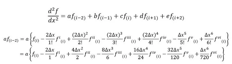
-
- The coefficients are calculated for all respective equations as follows ans plotted into taylors table as shown below:
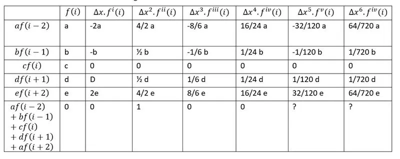
- with the help of equations obtained from the above table, we can calculate the values of each constants (a=-0.0833,b=1.3333,c=-2.5,d=1.333,e=-0.083330)
- from the values of constants we can conclude that the second last column of taylor table comes out to be zero and thus we finally get an equation:

- the term with power of deltax = 4 is ignored, thus the truncation error is a fourth order error.
- right-skewed scheme:
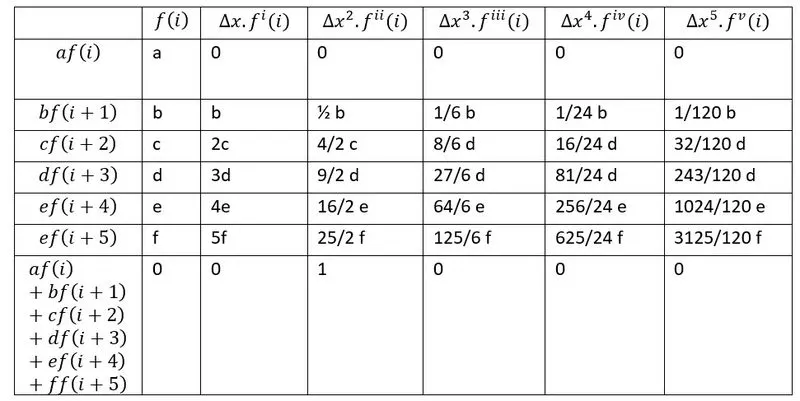
-
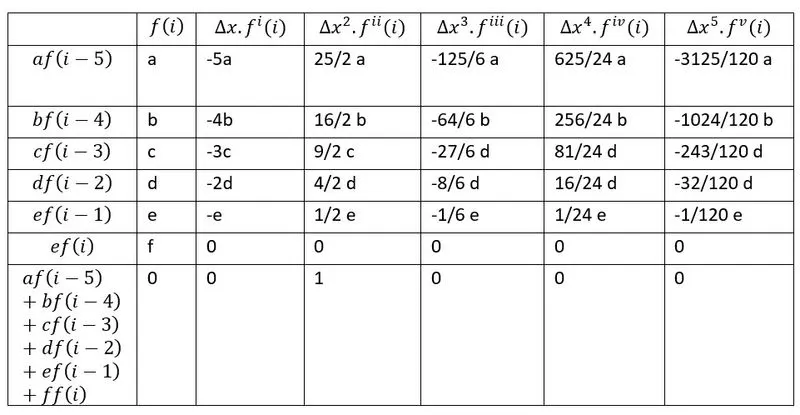
- similar process is followed as specified in the above discussion to calculate taylor table values
- left-skewed scheme:
- Matlab programming:
- defining the constants and exact derivative:
-
clear all
close all
clc

x=pi/3;
dx=linspace(pi/10,pi/10000,100);

%exact derivative
exact_derivative= -2*exp(x)*sin(x);
-
- programming the central differencing scheme:
- first the matrices are defined and the value of matrix B is calculated
- Next step is to calculate the central differencing approaximation usinng a for loop over a range of dx;
- finally an absolute error is calculated between exact and approaximated value
-
%Central differencing scheme
%calculating values of coefficients
A=[1 1 1 1 1; -2 -1 0 1 2; 4/2 1/2 0 1/2 4/2; -8/6 -1/6 0 1/6 8/6; 16/24 1/24 0 1/24 16/24];
C=[0;0;1;0;0];
B=AC;
%calculating second order derivative
% (a*f(x-2dx)+b*f(x-dx)+c*f(x)+d*f(x+dx)+e*f(x+2dx))/dx^2
for i=1:length(dx);
central_differencing(i) = ((B(1)*(exp(x-(2*dx(i)))*cos(x-(2*dx(i)))))+(B(2)*(exp(x-dx(i))*cos(x-dx(i))))+(B(3)*(exp(x)*cos(x)))+(B(4)*(exp(x+dx(i))*cos(x+dx(i))))+(B(5)*(exp(x+(2*dx(i)))*cos(x+(2*dx(i))))))/(dx(i)^2);
error_central_differencing(i) = abs(central_differencing(i)-exact_derivative);
end
- programming the right skewed scheme:
- using similar steps as mentioned for central differencing
-
%Right-Skewed Scheme
%calculating values of coefficient for right skewed scheme:
D=[1 1 1 1 1 1;0 1 2 3 4 5;0 1/2 4/2 9/2 16/2 25/2;0 1/6 8/6 27/6 64/6 125/6; 0 1/24 16/24 81/24 256/24 625/24; 0 1/120 32/120 243/120 1024/120 3125/120];
F=[0;0;1;0;0;0];
E=DF;
%calculating second order derivative
for i=1:length(dx)
right_skewed(i) = (E(1)*exp(x)*cos(x)+E(2)*exp(x+dx(i))*cos(x+dx(i))+E(3)*exp(x+2*dx(i))*cos(x+2*dx(i))+E(4)*exp(x+3*dx(i))*cos(x+3*dx(i))+E(5)*exp(x+4*dx(i))*cos(x+4*dx(i))+E(6)*exp(x+5*dx(i))*cos(x+5*dx(i)))/(dx(i)^2);
error_right_skewed(i) = abs(right_skewed(i)-exact_derivative);
end
- programming the left skewed scheme:
-
%Left Skewed Scheme
%calculating values of coefficient for left skewed scheme:
G=[1 1 1 1 1 1;-5 -4 -3 -2 -1 0; 25/2 16/2 9/2 4/2 1/2 0; -125/6 -64/6 -27/6 -8/6 -1/6 0; 625/24 256/24 81/24 16/24 1/24 0;-3125/120 -1024/120 -243/120 -32/120 -1/120 0];
I=[0;0;1;0;0;0];
H=GI;
%calculating second order derivative
for i=1:length(dx)
left_skewed(i) = (H(1)*exp(x-5*dx(i))*cos(x-5*dx(i))+H(2)*exp(x-4*dx(i))*cos(x-4*dx(i))+H(3)*exp(x-3*dx(i))*cos(x-3*dx(i))+H(4)*exp(x-2*dx(i))*cos(x-2*dx(i))+H(5)*exp(x-dx(i))*cos(x-dx(i))+H(6)*exp(x)*cos(x))/(dx(i).^2);
error_left_skewed(i) = abs(left_skewed(i)-exact_derivative);
end
-
- plotting the comparison of the error of all three schemes using loglog command:
-
figure(1) loglog(dx,error_central_differencing,'r'); hold on loglog(dx,error_right_skewed,'b'); loglog(dx,error_left_skewed,'g'); hold off legend('central differencing error','right skewed error','left skewed error'); xlabel('range of dx') ylabel('numerical error') title('Error comparison in discretization methods') 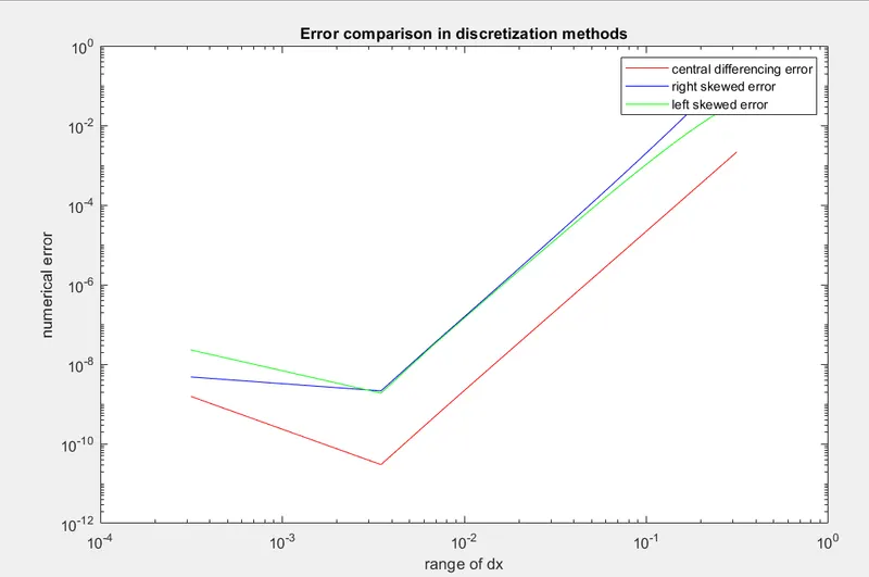
-
- defining the constants and exact derivative:
- conclusion: From the plot of numerical error vs range of dx for central differencing, right skewed and left skewed scheme we can conclude the following:
- the error in all three schemes decrease as the grid size reduces.
- The error in case of central differencing is least as compared to right skewed and left skewed schemes.