Week 9 - FVM Literature Review

FVM:-

FVM is a type of method which is used to solve the governing equations numerically by evaluating the surface integral of the finite volume.

In FVM instead of writing equations at a single point, equations are written in an entire finite volume. It means no assumptions are made over the shape of the volume. Inside the finite volume, all the terms are conserved.

Steps:-

1. The integral form of G.D.E.
2. Apply Gauss divergence theorem.
3. We get the discretized form which can be solved numerically

Consider 1-D steady-state heat conduction equation

`del/(delx)(alpha(delT)/(delx)) + S = 0`

S is source term

`alpha` is thermal diffusivity

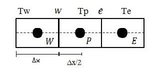
let P be the owner cell centroid and W, E is the neighbor cells centroid

Governing equation is valid at every point in the domain, which means it also valid in the entire control Volume.

`int(del/(delx)(alpha(delT)/(delx)) +S)dv = 0`

`intdel/(delx)(alpha(delT)/(delx))Adx +intSdv = 0`

on further simplification

`alphaA[(T_e -T_p)/(trianglex)] - alphaA[(T_p-T_w)/(trianglex)] +(S_u +S_pT_p)dv = 0`

i.e., The amount of heat that is removed from CV is conserved.

Finite Difference Method:-

It is a type of numerical method which is used to solve the governing equations numerically by using linear grid points.

Cons:-

1. we cannot use this method when grid points are not aligned properly along with their corresponding axis directions. These may occur due to complex geometry shapes.
2. As it not aligned properly we cannot calculate the properties at the next adjacent point exactly, but we can add some correction factor and approximate it, this method is called the Variable Transformation Method.
3. VTM is very complex to implement and requires a lot of computational effort.
4. For complex profiles, this method is less preferred.

Finite Volume Method:-

FVM is a type of method which is used to solve the governing equations numerically by evaluating the surface integral of the finite volume.

Pros:-

1. This method is conservative, as we are dealing with the surface integrals of finite volume.
2. Can be easily formulated for the unstructured meshes also.

Interpolation schemes:-

Interpolation schemes are used to find the values at the control faces of the cells because sometimes it is required for the evaluation of surface and volume integrals

For example:-

`d/dx(rhouphi) = d/dx(Gamma(dphi)/(dx))`

`phi` is a solution variable (scalar)

`(rhouphi)_e - (rhouphi)_w = (Gamma(dphi)/(dx))_e-(Gamma(dphi)/(dx))_w`

Evaluation of left hand side of above equation requires the values of `phi` over faces e and w. These values are estimated by using interpolation schemes.

• Upwind interpolation
• Linear interpolation
• QUICK scheme
• Hybrid( Mixture of upwind linear)
• TVD scheme

Flux Limiters:-

while calculating the variable gradients the solutions are not bounded and keep oscillating this occur due to discontinuity having a flux limiter will help to bound the gradient value thereby giving the stable solution.

Flux limiters operate as a switch and tune the numerical fluxes obtained from lower-order schemes and higher-order schemes. such that near the discontinuity lower order(stable) scheme is employed and away from it higher-order(accurate) scheme is employed.

let Flux at face e is calculated using a Higher-order scheme and lower-order scheme.

`F_e = L_e +psi(r)(H_e - L_e)`

`psi(r)` is flux limiter function and it depends on the smoothness parameter r.

`r_p = (phiP- phiW)/(phiE -phiP)`

The range of flux limiter is 0-1. 0 near discontinuities and a value of 1 away from them