Week 7 - Simulation of a 1D Super-sonic nozzle flow simulation using Macormack Method
AIM :- The main aim of this project is to simulate the isentropic flow through a quasi 1D subsonic-supersonic nozzle, by using MacCormack's technique for conservative form and Non-conservative form.
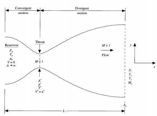
Description:-
Mathematically conservative and non-conservative forms are similar but numerically both the forms behaves differently depending on the type of the equations. As we are solving in one- dimensional we will concentrate only on the one-dimensional Governing equations for both the forms.
The choice of time step `trianglet` depends on the CFL condition which is C <= 0.5
`trianglet = c(trianglex)/(sqrtT +V)`
it returns an array of elements we consider the minimum value in it in order to get the stable steady solution.
First we will look into the Non-conservative form,
D.E'qs in Non-conservative form:-
continuity equation:-
`(delrho')/(delt') = -rho'(delV')/(delx') - rho'V'(del(lnA'))/(delx') - V'(delrho')/(delx')`
where V', `rho'`, A' ,x' are Non dimensional values
Momentum equation:-
`(delV')/(delt') = -V'(delV')/(delx') - 1/gamma((delT')/(delx') +(T')/(rho')(delrho')/(delx'))`
Energy equation:-
`(delT')/(delt') = -V'(delT')/(delx') - (gamma-1)T'[(delV')/(delx') +V'(del(lnA'))/(delx')]`
Here all the prime parameters are Dimensionless variables
we can use dimensional values as well the advantage of using dimensionless variables is that they vary in the range of 0 to 1 and it gives the ease of solving numerical problem.
- `x' = x/L,`
- `V' = V/a_o, a_o =sqrt(gammaRT_o)` `a_o` = speed of sound in reservoir
- `t' = t/(L/a_o)`
- `A' = A/(A^star)` `A^star` = sonic throat area.
After setting the governing equations we will set the initial conditions for density, Temperature and velocity at time step 0 seconds.
`rho = 1-0.3146x`
`T = 1 - 0.2314x`
`V = (0.1+1.09x)T^(1/2)`
x is local length on the CFD domain.
Predictor step:-
In predictor step we will use the forward difference for the spatial terms and the solution will be updated at every node say i. and this will be our predicted values
Corrector step :-
Using the predicted values we will do rearward difference to find the corrected values at every node i
In the end average of these two values will be used to find the final solution and it will be updated by intial conditions.
Boundary conditions:-
At node 1:-
`V_1 = 2V_2-V_3`
`rho_1 = 1`
`T_1 = 1`
At node N:-
`V_n = 2V_(n-1) -V_(n-2)`
`rho_n = 2rho_(n-1) -rho_(n-2)`
`T_n = 2T_(n-1) -T_(n-2)`
The choice of initial and boundary conditions are important for a solution to converge
D.E's in conservative form:-
The differentisal equations in these form are conserved.i.e.., All the quantities are in conserved form in other way all the quantities will be dependent on the spatial cordinate x or time.
Continuity equation:-
`(del(rho'A'))/(delt') + (del(rho'A'V'))/(delx') = 0`
Momentum equation :-
`(del(rho'A'V'))/(delt') +(del[rho'A'V'^2 +(1/gamma)p'A'])/(delx') = 1/gammap'(delA')/(delx')`
Energy equation:-
`(del[rho'((e')/(gamma-1)+gamma/2V'^2)A'])/(delt')+(del[rho'((e')/(gamma-1)+gamma/2V'^2)V'A' +p'A'V'])/(delx') = 0`
Unlike the Non-conservation form we can see that more dependent variables are present so it is not possible solve these equations directly but we can convert these eqautions into solution vectors
say,
U1 = `rho'A'`
U2 = `rho'A'V'`
U3 = `rho'((e')/(gamma-1)+gamma/2V'^2)A'`
F1 = `rho'A'V'`
F2 = `rho'A'V'^2 +(1/gamma)p'A'`
F3 = `rho'((e')/(gamma-1)+gamma/2V'^2)V'A' +p'A'V'`
J2 = `1/gammap'(delA")/(delx')`
using these we rewrite above D.E'qs
`(delU_1)/(delt') = -(delF_1)/(delx')`
`(delU_2)/(delt') = -(delF_2)/(delx') + J_2`
`(delU_3)/(delt') = -(delF_3)/(delx')`
Primitive variables are :-
`rho' = U_1/(A')`
`V' = U_2/U_1`
`T' = e' = (gamma-1)(U_3/U_1-gamma/2V'^2)`
`p' = rho'T'`
NOTE:- we need to update our primitive varibales for every timestep.
Let's make flux vector in terms of solution vectors in order to solve nemerically.
`F_1 = U_2`
`F_2 = U_2^2/U_1 +(gamma-1)/gamma(U_3 - gamma/2U_2^2/U_1)`
`F_3 = gamma(U_2U_3)/U_1 - (gamma(gamma-1))/2U_2^3/U_1^2`
`J_2 = (gamma-1)/gamma(U_3 - gamma/2U_2^2/U_1)(del(lnA'))/(delx')`
Boundary conditions:-
since the dependent variables are being solved by converted D.e'qs i.e.., U1, U2, U3 we need initial conditions for these same variables at time t = 0.
for `0<=x'<=0.5`
`rho' = 1.0`
`T' = 1.0`
for `0.5<=x'<=1.5`
`rho' = 1.0 -0.366(x'-0.5)`
`T' = 1.0 - 0.167(x'-0.5)`
for `1.5<=x'<=3.5`
`rho' = 0.634 - 0.3879(x'-1.5)`
`T' = 0.833 - 0.3507(x' - 1.5)`
`V' = U_2/(rho'A')`
At node 1:-
`U_(1(i=1)) =A'_(i=1)`
`U_(2(i=1)) = 2U_(2(i=2)) -U_(2(i=3)`
`U_3 = U_1((T')/(gamma-1) +gamma/2V'^2)`
At node n:-
`(U_1)_n = 2(U_1)_(n-1) - (U_1)_(n-2)`
`(U_2)_n = 2(U_2)_(n-1) - (U_2)_(n-2)`
`(U_3)_n = 2(U_3)_(n-1) - (U_3)_(n-2)`
MacCormack's technique:-
This is a one type of technique which is just like Lax-wendroff approach, explicit finite difference technique which is second order of accuracy in both spatial and time. The main advantage of this method is we will use simple first order difference only to get the second order accuracy.
This technique is a time marching solution based. we proceed to calculate the flow-field variables at the same grid points at time t+`deltat`
`rho_(i,j)^(t+trianglet) = rho_(i,j)^t +( (delrho)/(delt))_(avg) trianglet`
similar relations are written for the other flow-field variables also.
The arthimatic mean comprises of
`((delrho)/(delt))_(avg) = 1/2[((delrho)/(delt))_(i,j)^t + ((delrho)/(delt))_(i.j)^(t+trianglet)]`
The first term is the predictor step which is in forward difference and the following is corrector step which is rearward difference.
The corrector step is calculated by using the predictor step at every i,j node and final solution of second order accuracy.
Grid Independence:-
lets consider two cases 1 and 2 case 1 has the grid points of 31 and case 2 has grid points of 61
Grid independence is the condition at which there will be no significant changes in our numerical solution even when we increase the number of grid points in the domain
| Density | Temperature | Pressure | Mach number | |
| n = 31 | 0.6392 | 0.8364 | 0.5345 | 0.999 |
| n = 61 | 0.6386 | 0.8354 | 0.5324 | 1.000 |
| Exact | 0.634 | 0.833 | 0.528 | 1.000 |
from above table we can notice that there will be slight change in the values and its not going to effect the solution. Hence we can say that it is grid independent condition
Explanation of code:-
The main programm of the code consists of the variables like length of the domain L , number of nodes n, dx, number of time steps nt and so on.,
conservative and Non- conservative are the both functions which returns their corresponding primitive varibales like Densiity, velocity, Mach number , mass flow rate and pressure
Main programme:-
number of nodes,n = 31
length of domain, L = 3
gamma = 1.4
The area of the nozzle is a function of x only i.e.., at the throat the area is low.
and it follows the profile as shown in programme.
Consider a time steps of 1400
The two functions returns their corresponding values of density pressure mach number etc..,
i.e.., conservative and non- conservative
Different plots can be drawn by using these variables to compare solution.
clear all
close all
clc

n = 31;
x = linspace(0,3,n);
dx= x(2) - x(1);
gamma = 1.4;

%Area
a = 1 + 2.2*(x-1.5).^2;
throat = ((n-1)/2 +1);
%Time steps
nt = 1400;


%Conservation function

[rho, v, t, P, m, M, rho_t1,v_t1,P_t1,M_t1]= conservativeform(x,dx,a,nt,n,gamma,throat);


%Non-conservation function which returns the output density,velocity, temp
%as rho_n, t_n, v_n


[rho_n, v_n, t_n, P_n, m_n, M_n,rho_t2,v_t2,P_t2,M_t2] = nonconservative(x,dx,a,n,nt,gamma,throat);


%Plotting

%Timewise variation of different flow parameters conservative form
figure(2)
plot(linspace(1,nt,nt),rho_t1,'Linewidth',2)
hold on
plot(linspace(1,nt,nt),P_t1,'Linewidth',2)
plot(linspace(1,nt,nt),M_t1,'Linewidth',2)
legend('density','Pressure','Mach number')
title('Timewise variation of different flow parameters(Conservative form)')

%Timewise variation of different flow parameters Non-conservative form
figure(3)
plot(linspace(1,nt,nt),rho_t2,'Linewidth',2)
hold on
plot(linspace(1,nt,nt),P_t2,'Linewidth',2)
plot(linspace(1,nt,nt),M_t2,'Linewidth',2)
legend('density','pressure','Mach number')
title('Timewise variation of different flow parameters(Non-Conservative form)')

%Varition of mass flow rate in both forms
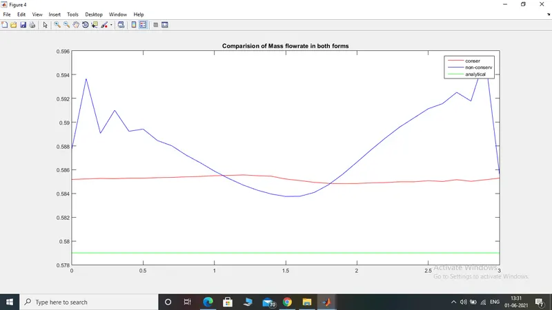
figure(4)
analyt = 0.579*ones(1,n);
plot(x,m,'r')
hold on
plot(x, m_n,'b')
plot(x, analyt,'g')
legend('conser','non-conserv','analytical')
title('Comparision of Mass flowrate in both forms')

%Steady state distribution of the flow variables in conservative form
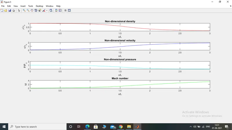
figure(5)
title(sprintf('steady-state distribution of flow field variables across the nozzle, no of time steps %d',nt))
subplot(5,1,1)
plot(x,rho,'r')
xlabel('x/L')
ylabel('rho/rho_o')
title('Non-dimensional density')

subplot(5,1,2)
plot(x, v,'b')
xlabel('x/L')
ylabel('v/v_o')
title('Non-dimensional velocity')

subplot(5,1,3)
plot(x, P, 'c')
xlabel('x/L')
ylabel('P/P_o')
title('Non-dimensional pressure')

subplot(5,1,4)
plot(x, M,'g')
xlabel('x/L')
ylabel('M')
title('Mach number')
Function:- Conservative form
function [rho, v, t, P, m, M,rho_t1,v_t1,P_t1,M_t1]= conservativeform(x,dx,a,nt,n,gamma,throat)

    %Setting initial density and temp values for a length of x
    for i = 1:n

        if x(i)>=0 && x(i)<=0.5
            rho(i) = 1;
            t(i) = 1;


        elseif x(i)>=0.5 && x(i)<= 1.5
            rho(i) = 1.0 - 0.366*(x(i)-0.5);
            t(i) = 1.0- 0.167*(x(i)- 0.5);

        else
            rho(i) = 0.634 - 0.3879*(x(i)-1.5);
            t(i) = 0.833 - 0.3507*(x(i) - 1.5);


        end


    end


     v = 0.59./(rho.*a);                %velocity
     P = rho.*t;                        %Pressure

    %Defining section vectors

    u1 = rho.*a;
    u2 = rho.*a.*v;
    u3 = rho.*((t./(gamma-1))+ ((gamma./2).*(v.^2))).*a;


    %Time loop
    for k = 1:nt

        u1_old = u1;
        u2_old = u2;
        u3_old = u3;

        %pure form of flux terms
        f1 = u2;
        f2 = ((u2.^2)./u1) + ((gamma-1)/gamma).*(u3 - ((gamma.*u2.^2)./(2.*u1)));
        f3 = ((gamma.*u2.*u3)./u1) - ((gamma*(gamma-1).*u2.^3)./(2.*u1.^2));

        %Time step based on cfl
        dt = min(0.5.*dx./(sqrt(t)+v));


        %Spatial loop predictor step

        for i = 2:n-1

            df1dx = (f1(i+1)-f1(i))/dx;
            df2dx = (f2(i+1)-f2(i))/dx;
            df3dx = (f3(i+1)-f3(i))/dx;
            J2(i) = (rho(i)*t(i)*(a(i+1)-a(i)))/(dx*gamma);

            %Continuity equation
            du1dt_p(i) = -df1dx;

            %Momentum equation
            du2dt_p(i) = -df2dx + J2(i);

            %Energy equation
            du3dt_p(i) = -df3dx;

            %Solution update

            u1(i) = u1(i) + du1dt_p(i)*dt;
            u2(i) = u2(i) + du2dt_p(i)*dt;
            u3(i) = u3(i) + du3dt_p(i)*dt;

        end

            P = rho.*t;

            %Updating the primitive values
            rho = u1./a;
            v = u2./u1;
            t = (gamma-1)*(u3./u1 - (gamma.*v.^2)./2);

        f1 = u2;
        f2 = ((u2.^2)./u1) + ((gamma-1)/gamma).*(u3 - ((gamma.*u2.^2)./(2.*u1)));
        f3 = ((gamma.*u2.*u3)./u1) - ((gamma*(gamma-1).*u2.^3)./(2.*u1.^2));


   u1(1) = a(1);
            u2(1) = 2*u2(2) -u2(3);
            u3(1) = u1(1)*((t(1)/(gamma-1)) + (gamma*v(1)^2)/2);
            %v(1) = u2(1)/u3(1);


        %Corrector step
         for i = 2:n-1


            df1dx = (f1(i)-f1(i-1))/dx;
            df2dx = (f2(i)-f2(i-1))/dx;
            df3dx = (f3(i)-f3(i-1))/dx;

            J2(i) = (rho(i)*t(i)*(a(i)-a(i-1)))/(dx*gamma);

            %Continuity equation
            du1dt_c(i) = -df1dx;

            %Momentum equation
            du2dt_c(i) = -df2dx + J2(i);

            %Energy equation
            du3dt_c(i) = -df3dx;

         end

         du1dt = 0.5*(du1dt_p +du1dt_c);
         du2dt = 0.5*(du2dt_p +du2dt_c);
         du3dt = 0.5*(du3dt_p +du3dt_c);

         %Final solution update

         for j =2:n-1

             u1(j) = u1_old(j) + du1dt(j)*dt;
             u2(j) = u2_old(j) + du2dt(j)*dt;
             u3(j) = u3_old(j) + du3dt(j)*dt;
         end


           %Boundary condition
           u1(1) = a(1);
           u2(1) = 2*u2(2) -u2(3);
           u3(1) = u1(1)*((t(1)/(gamma-1)) + (gamma*v(1)^2)/2);


        u1(n) = 2*u1(n-1) - u1(n-2);
        u2(n) = 2*u2(n-1) - u2(n-2);
        u3(n) = 2*u3(n-1) - u3(n-2);


        %Primitive variables.
        rho = u1./a;
        v = u2./u1;
        t = (gamma-1)*((u3./u1) - (gamma/2).*v.^2);
        P = rho.*t;
        m = rho.*v.*a;      %Mass flowrate
        M = v./sqrt(t);     %Mach number

        %Finding the values at throat for every time step.
        rho_t1(k) = rho(throat);
        v_t1(k) = v(throat);
        P_t1(k) = P(throat);
        M_t1(k) = M(throat);
        m_t1(k) = m(throat);

        %Plotting
        figure(1)
        hold on;

        if k == 1
            plot(x,m,'b','linewidth',2)
            hold on
        else
        if  k == 100
            plot(x,m,'g','linewidth',2)
        else
        if k == 500
            plot(x,m,'r','linewidth',2)
        else
        if  k == 700
            plot(x,m,'m','linewidth',2)
        else
        if k == 1000
            plot(x,m,'c','linewidth',2)
        end
        end
        end
        end
        end
        grid on


        legend({'1 sec','100 sec','500 sec','700 sec','1000 sec','1400 sec'})
        xlabel('Non Dimensional length')
        ylabel('Mass flowrate')
        title('Conservative form')
    end


    end
Function :- Non- conservative form
function [rho_n, v_n, t_n, P_n, m_n, M_n, rho_t2,v_t2,P_t2,M_t2] = nonconservative(x,dx,a,n,nt,gamma,throat)


%Input values

rho_n = 1 - (0.3146*x);             %Density
t_n = 1 - (0.2314*x);               %Temperature
v_n = (0.1+1.09*x).*t_n.^0.5;      %velocity

dt = min(0.5.*dx./(sqrt(t_n)+v_n));

%Time Marching
for k = 1:nt

     rho_old = rho_n;
     v_old = v_n;
     t_old = t_n;

    %spatial Loop
    for j = 2:n-1

        %For predictor step

        drhodx = (rho_n(j+1)-rho_n(j))/dx;
        dvdx = (v_n(j+1)-v_n(j))/dx;
        dtdx = (t_n(j+1) - t_n(j))/dx;
        dlogadx = (log(a(j+1))-log(a(j)))/dx;

        %continuity equation
        drhodt_p(j) = (-rho_n(j)*dvdx)- (rho_n(j)*v_n(j)*dlogadx) - (v_n(j)*drhodx) ;

        %Momentum equation
        dvdt_p(j) = (-v_n(j)*dvdx)-(1/gamma)*(dtdx+(t_n(j)/rho_n(j))*drhodx);

        %Energy Equation
        dedt_p(j) = (-v_n(j)*dtdx) - (gamma-1)*t_n(j)*(dvdx + v_n(j)*dlogadx);

        %Solution update
        rho_n(j) =rho_n(j) + drhodt_p(j)*dt;
        v_n(j) =v_n(j) + dvdt_p(j)*dt;
        t_n(j) =t_n(j) + dedt_p(j)*dt;

    end

    %Corrector step

     for j = 2:n-1


        drhodx = (rho_n(j)-rho_n(j-1))/dx;
        dvdx = (v_n(j)-v_n(j-1))/dx;
        dtdx = (t_n(j) - t_n(j-1))/dx;
        dlogadx = (log(a(j))-log(a(j-1)))/dx;

        %continuity equation
        drhodt_c(j) = (-rho_n(j)*dvdx) -(rho_n(j)*v_n(j)*dlogadx) -(v_n(j)*drhodx) ;

        %Momentum equation
        dvdt_c(j) = (-v_n(j)*dvdx) -(1/gamma)*(dtdx+(t_n(j)/rho_n(j))*drhodx);

        %Energy Equation
        dedt_c(j) = (-v_n(j)*dtdx) - (gamma-1)*t_n(j)*(dvdx + v_n(j)*dlogadx);

     end

    drhodt = 0.5*(drhodt_p +drhodt_c);
    dvdt = 0.5*(dvdt_p+dvdt_c);
    dedt = 0.5*(dedt_p +dedt_c);

    %Final solution Update
    for i = 2:n-1
        rho_n(i) = rho_old(i) + drhodt(i)*dt;
        v_n(i) = v_old(i) + dvdt(i)*dt;
        t_n(i) = t_old(i) + dedt(i)*dt;
    end

    %Applying the Boundary conditions

    %inlet
    v_n(1) = (2*v_n(2)) - v_n(3);
    rho_n(1) = 1;
    t_n(1) = 1;


    %outlet
    v_n(n) = 2*v_n(n-1) - v_n(n-2);
    rho_n(n) = 2*rho_n(n-1) - rho_n(n-2);
    t_n(n) = 2*t_n(n-1) - t_n(n-2);

        P_n = rho_n.*t_n;
        m_n = rho_n.*v_n.*a;
        M_n = v_n./sqrt(t_n);

    %Values at throat
    rho_t2(k) = rho_n(throat);
        v_t2(k) = v_n(throat);
        P_t2(k) = P_n(throat);
        M_t2(k) = M_n(throat);
        m_t2(k) = m_n(throat);

end


end
Results:-
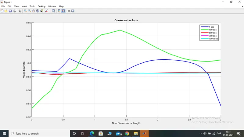
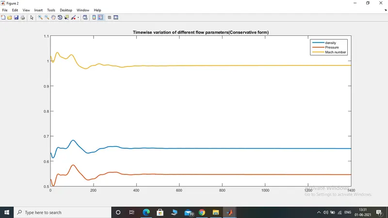
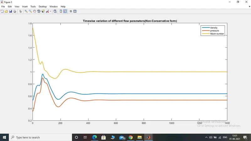
Conclusion:-
From the above results and plots it can be concluded that Numerically both the forms will be used but using the conservative form will lead closer results to the exact solution and also whenever if there shock wave problems only we will use conservative form.