Week 5.1 - Mid term project - Solving the steady and unsteady 2D heat conduction problem

General 2-D Heat conduction equation in Transient form

`(delT)/(delt)+alpha((del^2T)/(delx^2)+(del^2T)/(dely^2)) = 0`

For steady state:-

`(del^2T)/(delx^2)+(del^2T)/(dely^2) = 0`

For solving the steady state equation we can use any of the iterative techniques. i.e...,

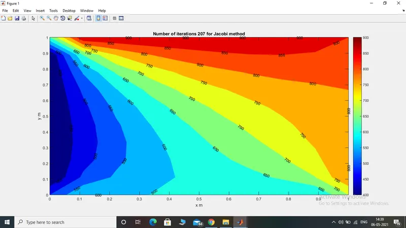
1. Jacobi method
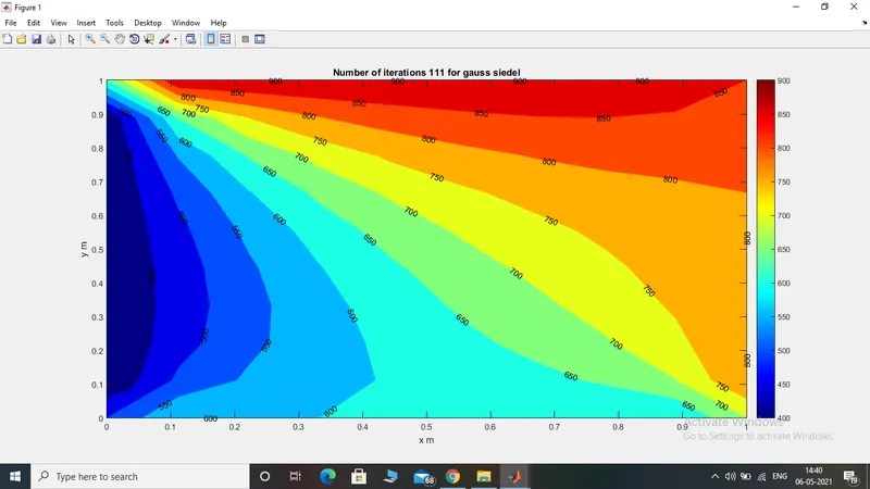
2. Gauss siedel method
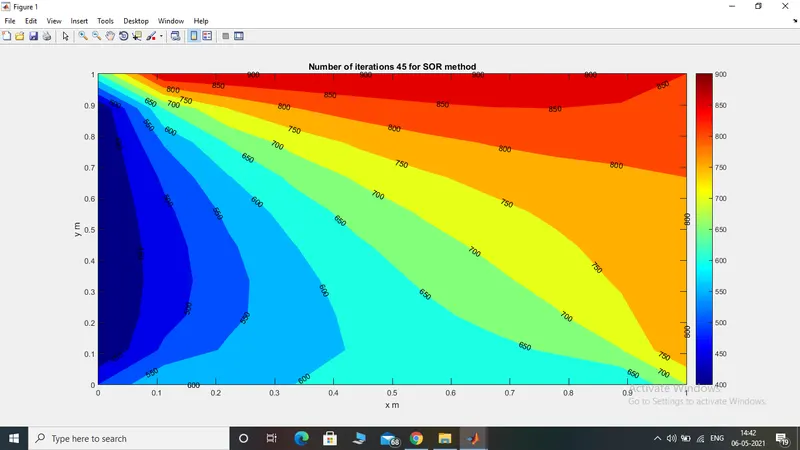
3. successive over relaxation method

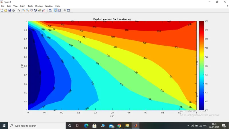
For Transient state we can solve it by Explicitly or implicitly. There is no need of iterative techniques to solve explicitly because all the values are at known timestep onle.

For implicit method we use each of the iterative methods as mentioned above and see the results.

The above differential form can be discretised by using approximation and can be written as

For steady state:-

`T(i,j) = 1/k((T(i-1,j)+T(i+1,j))/dx^2 +(T(i,j-1)+T(i,j+1))/dy^2)`

For unsteady:-

`T(i,j)=((Tprev(i,j))/(1+2k1+ 2k2))+ (Told(i-1,j)+Told(i+1,j)*k1(1+(2*k1)+ (2*k2))^-1) + (Told(i,j-1)+Told(i,j+1)*k2*(1+(2*k1)+ (2*k2))^-1)`

The above Tranient eq can be solved iteratively by using jacobi,gauss siedel and SOR methods.

Let nx ny be the number of nodes in the x and y direction.

x and y be the nx ny number of points between 0 to 1 of equal spacing. dx dy be the distance between the two nodes.

Now we will set initial boundary condition temperature values to the matrix of (nx x ny) which is top, left, bottom, right boundary.

choose your methods from 1 to 7 as

1. Jacobi steady
2. GS steady
3. SOR steady
4. Explicit Transient
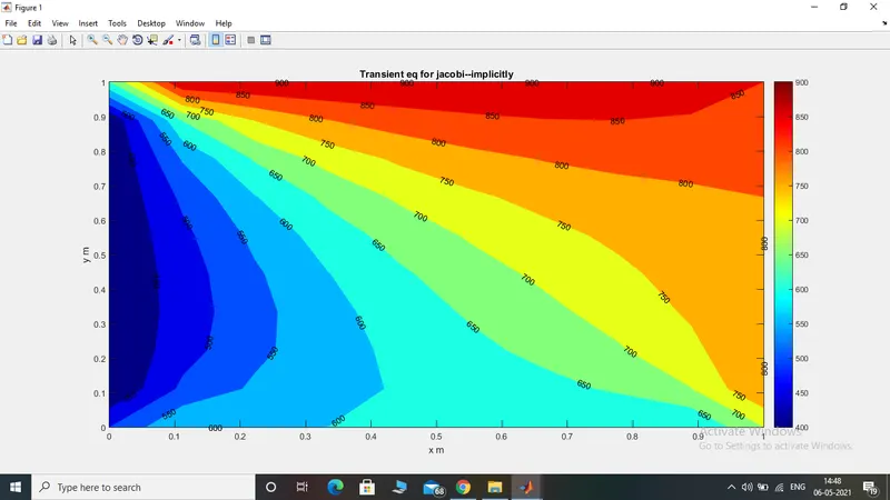
5. Implicit Transient jacobi
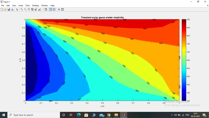
6. implicit Transient Gauss siedel
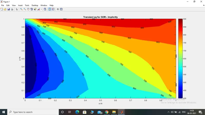
7. Implicit Transient SOR

The required variables are to be assigned in order to compute the solution in the above given formulae.

And for solving we have convergence loop to compute below the tolerance and then spatial loop.

Main Programme:-

clear all
close all
clc

%solution for the 2-D Heat conduction equation

nx = 10;
ny = 10;

x = linspace(0,1,nx);
y = linspace(0,1,ny);

dx = x(2)-x(1);
dy = y(2)-y(1);

%Initial temp 
%Boundary conditions temp values
T = ones(nx,ny)*300;

T(1,2:nx-1) = 600;      %Top boundary 600
T(2:ny-1,1) = 400;      %left boundary 400
T(end,2:nx-1) = 900;    %bottom boundary 900
T(2:ny-1,end) = 800;     %right boundary 800

%values at the corners 
T(1,1) = (T(1,2)+T(2,1))/2;
T(1,end) = (T(1,nx-1)+T(2,end))/2;
T(end,1) = (T(end-1,1)+T(end,2))/2;
T(end,end) = (T(end,end-1)+T(end-1,end))/2;

 
% For steady state eq 
%T(i,j) = 1/K * (T(i-1,j)+T(i+1,j)/dx^2 +T(i,j-1) +T(i,j+1)/dy^2)

K = 2*(dx^2 + dy^2)/(dx^2*dy^2);

%initial T
Told = T ;

tolerance = 1e-4;
Error1 = 1e9;
my_method = 7;

%Jacobi method 
jacobi_iter = 0;


if my_method == 1
    
    while Error1>tolerance
    
    %spatial loop
        for i = 2:nx-1
              for j = 2:ny-1
               Term1 = (Told(i-1,j)+Told(i+1,j))/dx^2;
               Term2 = (Told(i,j-1)+Told(i,j+1))/dy^2;
               T(i,j)=1/K*(Term1 + Term2);
              end
        end
    
        Error = max(abs(T-Told));
        Error1 = max(Error);

        %update the old temp values
        Told = T;

        jacobi_iter = jacobi_iter +1;
        
        %simulation plot
        contourf(x,y,T,'ShowText','on','linecolor','non')
        str = sprintf('Number of iterations %d for Jacobi method',jacobi_iter);
        title(str)
        xlabel('x m')
        ylabel('y m')
        colormap(jet(256))
        colorbar
        pause(0.03)
    end
end
    
% Gauss siedel method

if my_method == 2
    Gauss_iter = 0;
    while Error1>tolerance
    
    %spatial loop
    for i = 2:nx-1
        for j = 2:ny-1
           Term1 = (T(i-1,j)+Told(i+1,j))/dx^2;
           Term2 = (T(i,j-1)+Told(i,j+1))/dy^2;
           T(i,j) = 1/K *(Term1+Term2);
        end
    end
    
    Error = max(abs(T-Told));
    Error1 = max(Error);
    
    %update the old temp values
    Told = T;
    
    Gauss_iter = Gauss_iter +1;
    %simulation plot
    contourf(x,y,T,'ShowText','on','linecolor','non')
    str = sprintf('Number of iterations %d for gauss siedel',Gauss_iter);
    title(str)
    xlabel('x m')
    ylabel('y m')
    colormap(jet(256))
    colorbar
    pause(0.03)
    end
end

%For SOR method 
omega = 1.4;

if my_method == 3
    sor_iter = 0;
    while Error1>tolerance
    
    %spatial loop
        for i = 2:nx-1
            for j = 2:ny-1
             Term1 = (T(i-1,j)+Told(i+1,j))/dx^2;
             Term2 = (T(i,j-1)+Told(i,j+1))/dy^2;
             T(i,j) = 1/K *(Term1+Term2);
             T(i,j) = Told(i,j)*(1-omega) + omega*(T(i,j));
            end
        end
    Error = max(abs(T-Told));
    Error1 = max(Error);
    
    %update the old temp values
    Told = T;
    sor_iter = sor_iter +1;
    
    %simulation plot
    contourf(x,y,T,'ShowText','on','linecolor','non')
    str = sprintf('Number of iterations %d for SOR method',sor_iter);
    title(str)
    xlabel('x m')
    ylabel('y m')
    colormap(jet(256))
    colorbar
    pause(0.03)
    end
end

%%2-D equation for transient state 

%Explicit method

dt = 0.001;             %Timestep
alpha = 1.6;            %Thermal Diffusivity
k1 = (alpha*dt/dx^2);
k2 = (alpha*dt/dy^2);
Tprev = T;

if my_method == 4
    %Time loop
    for k = 1:1400    
        %spatial loop
            for i = 2:nx-1
                for j = 2:ny-1
                    term1 = Told(i-1,j)-(2*Told(i,j))+Told(i+1,j);
                    term2 = Told(i,j-1)-(2*Told(i,j))+Told(i,j+1);
                    T(i,j)=Tprev(i,j)+(k1*term1)+(k2*term2);
                end
            end            
            
            %Update the old velocities 
            Told = T;
        
            %update the previous time step T
            Tprev = T;
    
     
    %simulation plot 
    contourf(x,y,T,'ShowText','on','linecolor','non')
    title('Explicit method for transient eq')
    xlabel('x m')
    ylabel('y m')
    colormap(jet(256))
    colorbar
    pause(0.03)
    
   end
    
end


if my_method == 5
    %Time loop
    for k = 1:1400
        Error1 = 1e9;    
        while Error1>tolerance
        %spatial loop
            for i = 2:nx-1
                for j = 2:ny-1
                    term1 = (1+(2*k1)+ (2*k2))^-1;
                    term2 = Told(i-1,j)+Told(i+1,j);
                    term3 = Told(i,j-1)+Told(i,j+1);
                    T(i,j)=(Tprev(i,j)*term1)+ (term2*k1*term1) + (term3*k2*term1);
                end
            end  
            Error = max(abs(T-Told));
            Error1 = max(Error);
            
            %Update the old velocities 
            Told = T;
        end   
            %update the previous time step T
            Tprev = T;
    
     
    %simulation plot 
    contourf(x,y,T,'ShowText','on','linecolor','non')
    %set(gca,'ydir','reverse')
    
    title('Transient eq for jacobi--implicitly')
    xlabel('x m')
    ylabel('y m')
    colormap(jet(256))
    colorbar
    pause(0.03)
    
    end
    
end

%Gauss siedel method 
if my_method == 6 
    %Time loop
    for k = 1:1400
        Error1 = 1e9;
        
        while Error1>tolerance
        %spatial loop
            for i = 2:nx-1
                for j = 2:ny-1
                    term1 = (1+(2*k1)+ (2*k2))^-1;
                    term2 = T(i-1,j)+Told(i+1,j);
                    term3 = T(i,j-1)+Told(i,j+1);
                    T(i,j)=(Tprev(i,j)*term1)+ (term2*k1*term1) + (term3*k2*term1);
                end
            end  
            Error = max(abs(T-Told));
            Error1 = max(Error);
            
            %Update the old velocities 
            Told = T;
        end   
            %update the previous time step T
            Tprev = T;
    
     
    %simulation plot 
    contourf(x,y,T,'ShowText','on','linecolor','non')
    title('Transient eq by gauss siedel--implicitly')
    xlabel('x m')
    ylabel('y m')
    colormap(jet(256))
    colorbar
    pause(0.03)
    
    end
    
end

%Successive over relaxation method
if my_method == 7 
    %Time loop
    for k = 1:1400
        Error1 = 1e9;
        
        while Error1>tolerance
        %spatial loop
            for i = 2:nx-1
                for j = 2:ny-1
                    term1 = (1+(2*k1)+ (2*k2))^-1;
                    term2 = T(i-1,j)+Told(i+1,j);
                    term3 = T(i,j-1)+Told(i,j+1);
                    T(i,j)=(Tprev(i,j)*term1)+ (term2*k1*term1) + (term3*k2*term1);
                    T(i,j) = (Told(i,j)*(1-omega)) + omega*(T(i,j));
                end
            end  
            Error = max(abs(T-Told));
            Error1 = max(Error);
            
            %Update the old velocities 
            Told = T;
        end   
            %update the previous time step T
            Tprev = T;
    
     
    %simulation plot 
    contourf(x,y,T,'ShowText','on','linecolor','non')
    title('Transient eq for SOR-- Implicitly')
    xlabel('x m')
    ylabel('y m')
    colormap(jet(256))
    colorbar
    pause(0.03)
    
    end
    
end

Results:-

Conclusion:-

From the above results it is observed that the number of iterations takes to reach the steady sate is more for the jacobi. and less for the sor

• Jacobi > Gauss siedel >SOR