Week 3.5 - Deriving 4th order approximation of a 2nd order derivative using Taylor Table method

let's write the given function f = exp(x)*cos(x) in a function file

Function

function result = f(x)
result = exp(x)*cos(x);
end

First find the coefficient matrix to compute the coefficients a,b,c,d,e in central difference scheme, by using taylor table method coeff matrix A is obtainned and calculate the coefficients by matrix inversion of A

substitute the coefficients in below eq to get the seond order approximation at x

d^2f/dx^2 = af(i-2)+bf(i-1)+cf(i)+df(i+1)+ef(i+2) / dx^2 ----- Central difference

then find the error between the analytical derivative of f(x) and numerical derivative of f(x)

similarly for left skewed and right skewed schemes also calculate the coefficient matrixes and calculate the second order derivative and calculate their corresponding errors

• af(i-5)+bf(i-4)+cf(i-3)+df(i-2)+ef(i-1)+ff(i) / dx^2 ------ Left skewed scheme
• af(i)+bf(i+1)+cf(i+2)+df(i+3)+ef(i+4)+ff(i+5) / dx^2------Right skewed scheme

All the above schemes are fourth order accuracy i.e.., In Central difference scheme we will have 5 unknowns and we will use 5 equations to solve, as we are doing for the second order derivative except the second order term remaining 4 terms are zero and 6 term is also zero by substituting the coefficients and remaining 7 term which is order of 6 will divided by the dx^2 and its fourth order accuracy

In left and right skewed we have 6 unknowns, by following the same as mentioned above 7 term is of power 6 divided by dx^2 and is of order 4

Central difference scheme approximate the solution by taking left and right side of the current point and it's not possible at the boundaries of the stencil i.e.., right end or left end. In that case we will use either left skewed or right skewed scheme to solve

Main program

clear all
close all
clc

%second order derivative of function f(x) with fourth order accuracy 
x = pi/3;
fx = -2*exp(x)*sin(x);
dx = pi/60;

%Taylor table method for fourth order accuracy with CD scheme
%d^2/dx^2 = af(i-2)+bf(i-1)+cf(i)+df(i+1)+ef(i+2) / dx^2
%coefficient matrix obtained by using central difference scheme 
A = [ 1        1     1   1       1 ;
     -2       -1     0   1       2 ;
      2        1/2   0   1/2     2 ;
     -8/6     -1/6   0   1/6     8/6;
      16/24    1/24  0   1/24    16/24 ];
 
 B = [ 0; 0; 1; 0; 0];
 
 X = inv(A)*B;
 
 f1 = (X(1)*f(x-2*dx)+X(2)*f(x-dx)+X(3)*f(x)+X(4)*f(x+dx)+X(5)*f(x+2*dx))/dx^2;
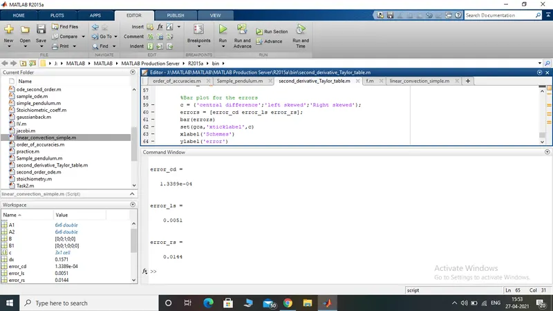
 error_cd = abs(f1-fx)
 
 %Coefficient matrix obtained by using skewed left sided difference
 
  A1 = [ 1              1        1             1        1      1;
      -5             -4        -3            -2      -1      0;
      25/2           16/2       9/2         4/2      1/2     0;
      -125/6        -64/6       -27/6       -8/6    -1/6     0;
      625/24         256/24      81/24       16/24   1/24    0;
      -3125/120      -1024/120   -243/120    -32/120 -1/120  0];
 
  B1 = [ 0; 0; 1; 0 ; 0; 0];
  
  Y = inv(A1)*B1;
  
  f2 = (Y(1)*f(x-5*dx)+Y(2)*f(x-4*dx)+Y(3)*f(x-3*dx)+Y(4)*f(x-2*dx)+Y(5)*f(x-dx)+Y(6)*f(x))/dx^2;
  
  error_ls = abs(fx-f2)
  
  %coefficient matrix for skewed right sided difference by using Taylor
  %table
  
  A2 = [ 1      1       1       1       1       1;
         0      1       2       3       4       5;
         0      1/2     2       9/2     16/2    25/2;
         0      1/6     8/6     27/6    64/6    125/6;
         0      1/24    16/24   81/24   256/24  625/24;
         0      1/120   32/120  243/120 1024/120 3125/120];
     
    z = inv(A2)*B1;
     
    f3 = (z(1)*f(x)+z(2)*f(x+dx)+z(3)*f(x+2*dx)+z(4)*f(x+3*dx)+z(5)*f(x+4*dx)+z(6)*f(x+5*dx))/dx^2;
    error_rs = abs(fx-f3)
    
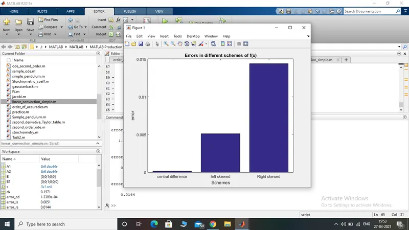
    %Bar plot for the errors
    c = {'central difference';'left skewed';'Right skewed'};
    errors = [error_cd error_ls error_rs];
    bar(errors)
    set(gca,'xticklabel',c)
    xlabel('Schemes')
    ylabel('error')
    title('Errors in differenr schemes of f(x)')

output:- Errors in different schemes when comparing with analytical derivative

plot:-