Week 9 - FVM Literature Review
Finite Volume Method - Basic Introduction
From a physical point of view, Finite Volume Method is based on the balancing the fluxes through control volumes and from a numerical point of view, FVM is the generalisation of FDM in a geometrical and topological perspective. Implementation of FVM enabled the conservation of quantities at the discretized level which is much more accurate than the non-conservative forms.
| S. No | Finite Difference Method | Finite Volume Method |
| 1. | Geometries are represented by structured grids and computation is carried out for every node. | FVM can be employed over structured as well as unstructured grids in a geometry. the properties are computed over an entire cell rather than the node points alone in the case of FDM |
| 2. | Approximations are computed using Taylor's series | Approximations of the closed integrals of the values in a finite cell is computed |
| 3. | The governing equations are represented in the differential form | The divergence of the govering equations are represented in a conservative form. |
Interpolation Schemes
These schemes are used to transform cell-centre quantities to the face centres of the respective cell in a finite volume method.
To understand better, let us define two cells named as owner(P) and neighbouring(N) cells. Assuming we know the value of any field variable(p,T or U) defined generally by `phi`. `phi undersetp`and `phi undersetn`are the known variables at the centroids of the respective cells and `phi undersetf`is the value of the variable to be computed at the cell face. The field variables or mass flux are assumed to flow from the left to right.
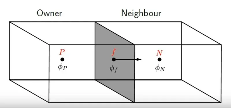
1. Linear/Central Differencing Scheme
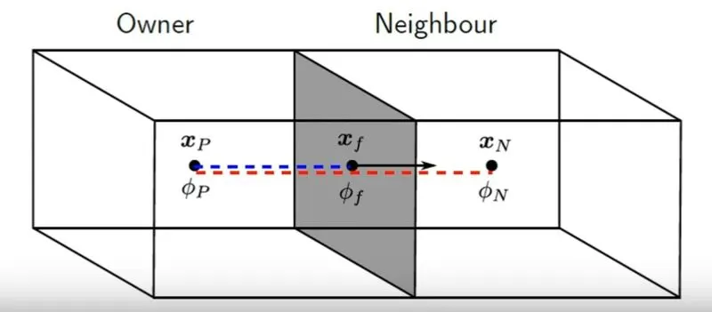
`underset(f)(phi) = psi*underset(N)(phi) + (1-psi)*underset(P)(phi)`
where `psi = (abs(underset(f)(x)-underset(P)(x)))/(abs(underset(N)(x)-underset(P)(x)))`
`underset(f)(x), underset(P)(x) and underset(N)(x)`are the centroids of the face and cells respectively
This scheme is second order accurate and the variation is linear in nature. It results in accuracy but stability is not always guaranteed as this scheme is unbounded in nature.
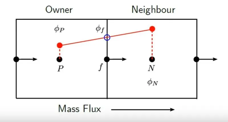
2. Upwind Differencing Scheme
It is important to define the mass flux in this case. The mass flux through a cell is given by the formula below
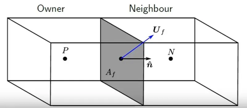
`underset(f)(F) = underset(f)rho*underset(f)A*(underset(f)U*hatn)`
The value of `underset(f)phi = {(underset(P)phi,underset(f)F>0),(underset(N)phi,underset(f)F<0):}`
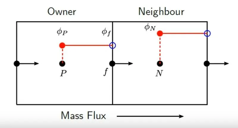
This scheme is basically a projection of field variables onto the cell face. `phi`no longer varies linearly across the cell face and is a constant between the cell centroid and face.This scheme is only first order accurate and is a stable scheme for convection dominated problem statements.
3.Linear Upwind Differencing
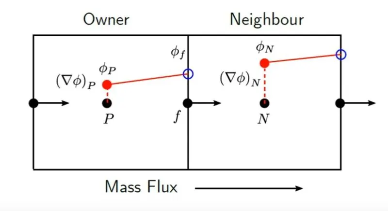
It is a popular scheme whcih combines the previous 2 schemes and is more accurate than the upwind scheme.The cell face is defined as given below
`underset(f)phi = {(underset(P)phi+(nabla*underset(P)phi)*hatr;underset(f)F>0),(underset(N)phi+(nabla*underset(N)phi)*hatr;underset(f)F<0):}`
A gradient of the variable `nablaphi`is used to improve the accuracy of the extrapolation.The variation of `phi`is linear and no longer constant and the scheme is second order accurate.
4. Advanced Differencing Schemes
Advanced solvers use a combination of
a. Linear/Central differencing for accuracy `underset(CD)phi`
b. Upwind differencing for stability `underset(UD)phi`
It is given by the general defintion
`underset(f)phi = psi*underset(UD)phi+(1-psi)*underset(CD)phi`
where `psi`is a blending function `0<=psi<=1`to switch between schemes.
Gradient/Flux Limiters
Usage of linear or linear upwind schemes which are unbounded sometimes may result in the interpolation or extrapolation of field variables to the cell face which are numerically greater than the known field variables in the centroid of the neighbouring cell. This results in an inaccurate solution eventually and we use flux or gradient limiters to restrict the gradients (`nabla underset(P)phi or nabla underset(N)phi`) to prevent local maxima/minima.
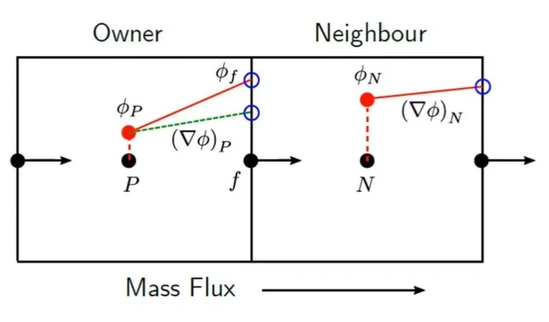
Therefore the field variable on the cell is controlled by a factor `psi`ranging between 0 and 1 and is given as
`underset(f)phi = {(underset(P)phi+psi*(nablaunderset(P)phi)*hatr; underset(f)F>0),(underset(N)phi+psi*(nablaunderset(N)phi)*hatr; underset(f)F<0):}`