Week 5 - Mid term project - Solving the steady and unsteady 2D heat conduction problem

The problem considered here is a two dimensional heat conduction equation with solutions for both the steady and transient state conditions. The iterative techniques such as Jacobi, Gauss-Siedal iterations and also Successive Over Relaxation(SOR) employed over the former two techniques are used to arrive at the solution. The transient state equation is solved using explicit as well as implicit schemes. The implicit scheme is worked out using iterative techniques in the time marching procedure.

A 1x1 square grid consisting of nx nodes along x-axis and ny nodes along y-axis is initialized.

A function temp_matrix(t,b,l,r,nx,ny) is defined to assign boundary conditions to the square grid with temperatures at the top(t), bottom(b) , left(l) and right(r) boundaries. The temperatures at the vertices of the grid are taken as the average of the temperatures of the corresponding boundaries/sides. The variables are as follows; nx = 10, ny = 10, t = 600, b = 900, l = 400, r = 800.The temperatures at all other nodes are assigned the value of 500K which is the initial condition.

Steady State Analysis

(d^2T/dx^2)+(d^2T/dy^2) = 0

The steady state analysis is performed by employing iterative techniques such as Jacobi, Gauss-Siedal and Successive Over Relaxation(SOR) over Jacobi and Gauss-Siedal approaches in MATLAB.

1. The Jacobi iterative technique uses the previous generation of temperature values to compute the next generation even if the an updated value exists in the computational matrix. Hence the number of iterations taken to reach the final solution in this method is significantly higher than other techniques.

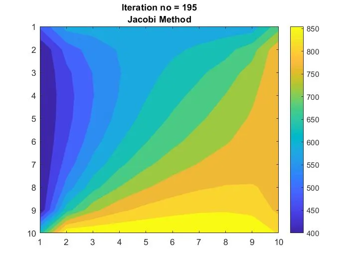
2. The Gauss-Siedal iterative technique uses the updated values if available to calculate the next generation of values in the computational matrix. Due to this approach used in the Gauss-Siedal technique, the number of iterations are lesser as compared to Jacobi technique and hence the solution is converged at a faster rate.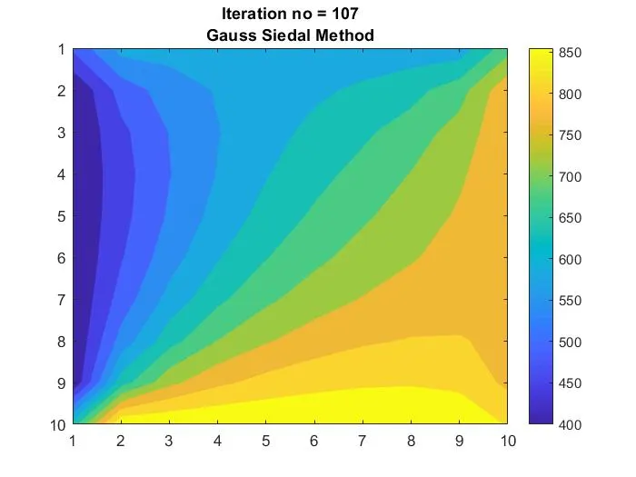

1. The Successive Over Relaxation (SOR) technique is an add-in function which can be used to fine tune the above mentioned Jacobi and Gauss-Siedal iterative techniques. A trial and error approach is used to vary the alpha parameter 'a' in order to arrive at the least number of iterations.

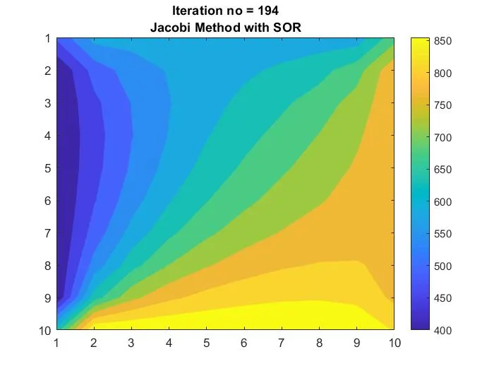
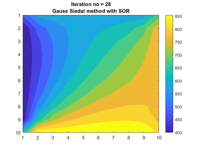
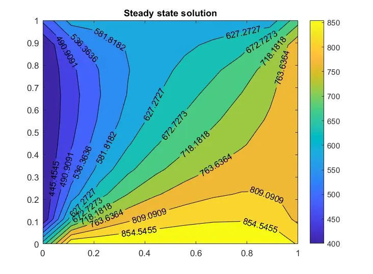
   clear all
   close all
   clc
   
   %steady state 2d heat conduction equation (d^2T/dx^2)+(d^2T/dy^2)=0
   
   %2d space grid
   nx = 10;
   ny = 10;
   x = linspace(0,1,nx); dx = x(3)-x(2);
   y = linspace(0,1,ny); dy = y(3)-y(2);
   
   k1 = (2*(dx^2+dy^2))/dy^2; 
   k2 = (2*(dx^2+dy^2))/dx^2;
   
   %2d temperature grid
   T = temp_matrix(600,900,400,800,nx,ny);%defined function
   T_old = T;
   
   error = 9e9;
   tolerance = 1e-4;
   
   iteration_no = 1;
   iter = 1;
   
   %convergence loop
   if iter == 1 %Jacob iteration
       while(error>tolerance)
       %space loop
           for i = 2:ny-1
               for j = 2:nx-1
                   T(i,j) = ((T_old(i+1,j)+T_old(i-1,j))/k1)+((T_old(i,j-1)+T_old(i,j+1))/k2);
               end
           end
           iteration_no = iteration_no+1;
           error = max(max(abs(T-T_old)));
           T_old = T;
           figure(1)
           contourf(T,nx,'edgecolor','none');
           set(gca,'YDIR','reverse');
           title_text = sprintf('Iteration no = %d',iteration_no);
           title({title_text;'Jacobi Method'});
           pause(0.05);
       end
       figure(2) 
       [X,Y] = meshgrid(x,y);
       contourf(X,flipud(Y),T,nx,'ShowText','on'); 
       title('Steady state solution');
       colorbar;
   end
   
   %convergence loop
   if iter == 2 %Gauss-Seidal iteration
       while(error>tolerance)
       %space loop
           for i = 2:nx-1
               for j = 2:ny-1
                   T(i,j) = ((T_old(i+1,j)+T(i-1,j))/k1)+((T(i,j-1)+T_old(i,j+1))/k2);
               end
           end
           iteration_no = iteration_no+1;
           error = max(max(abs(T-T_old)));
           T_old = T;
           figure(3)
           contourf(T,nx,'edgecolor','none');
           set(gca,'YDIR','reverse');
           title_text = sprintf('Iteration no = %d',iteration_no);
           title({title_text;'Gauss Siedal Method'});
           pause(0.05);
       end
       figure(4) 
       [X,Y] = meshgrid(x,y);
       contourf(X,flipud(Y),T,nx,'ShowText','on');
       title('Steady state solution');
       colorbar;
   end
   
   %Successive Over Relaxation 
   
   %convergence loop
   if iter == 3 %Jacob iteration with SOR
       while(error>tolerance)
       %space loop
           for i = 2:nx-1
               for j = 2:ny-1
                   a = 1.01;
                   T(i,j) = T_old(i,j)*(1-a)+(a*(((T_old(i+1,j)+T_old(i-1,j))/k1)+((T_old(i,j-1)+T_old(i,j+1))/k2)));
               end
           end
           iteration_no = iteration_no+1;
           error = max(max(abs(T-T_old)));
           T_old = T;
           figure(5)
           contourf(T,nx,'edgecolor','none');
           set(gca,'YDIR','reverse');
           title_text = sprintf('Iteration no = %d',iteration_no);
           title({title_text;'Jacobi Method with SOR'});
           pause(0.05);
       end
       figure(6) 
       [X,Y] = meshgrid(x,y);
       contourf(X,flipud(Y),T,nx,'ShowText','on'); 
       title('Steady state solution');
       colorbar;
   end
   
   %convergence loop
   if iter == 4 %Gauss-Siedal with SOR
       while(error>tolerance)
       %space loop
           for i = 2:nx-1
               for j = 2:ny-1
                   a = 1.5;
                   T(i,j) = T_old(i,j)*(1-a)+(a*(((T_old(i+1,j)+T(i-1,j))/k1)+((T(i,j-1)+T_old(i,j+1))/k2)));
               end
           end
           iteration_no = iteration_no+1;
           error = max(max(abs(T-T_old)));
           T_old = T;
           figure(7)
           contourf(T,nx,'edgecolor','none');
           set(gca,'YDIR','reverse')%reversing y axis
           title_text = sprintf('Iteration no = %d',iteration_no);
           title({title_text;'Gauss Siedal method with SOR'});
           pause(0.05);
       end
       figure(8) 
       [X,Y] = meshgrid(x,y);
       contourf(X,flipud(Y),T,nx,'ShowText','on'); 
       title('Steady state solution');
       colorbar;
   end
   
   function solution = temp_matrix(t,b,l,r,nx,ny)
      
       T = 500*ones(ny,nx);
       T(1,2:nx-1) = t;%top
       T(ny,2:nx-1) = b;%bottom
       T(2:ny-1,1) = l;%left
       T(2:ny-1,nx) = r;%right
       T(1,1) = (t+l)/2; T(1,nx) = (t+r)/2; T(ny,1) = (l+b)/2; T(ny,nx) = (b+r)/2;%corners
       
       solution = T;
   end​

Transient State Analysis

(d^2T/dx^2)+(d^2T/dy^2) = (1/a)*(dT/dt)

The transient state analysis is performed using the explicit and implicit schemes using MATLAB.

Explicit Scheme:

In this approach, each difference equation contains only one unknown variable and hence can be solved explicitly in a straightforward manner. Setting up the program in this case is simple and does not use any of the iterative techniques within the explicit scheme. However, the stability criterion given by CFL no is to be followed else the solution becomes unstable and there is no convergence. The stability criterion generally demands the value of dt to be infinitesimally small and this in turn results larger number of timesteps to be computed leading to convergence at a slower rate.

Implicit Scheme:

In this approach, each difference equation contains more than one unknown variable and hence a series of algebraic equations have to be solved within each time step to determine the values of the unknown variable at the next time-step. The system of difference equations can be represented as a coefficient matrix in the form of a tridiagonal matrix which consists of non-zero elements along its three diagonals.

The advantage of the implicit scheme is that stability can be maintained over large values of dt which results in convergence achieved at a faster rate over a given interval of t. However, this scheme also presents its disadvantages wherein the iterative techniques are required within each time-step(in spite of lesser number of time-steps) which may result in larger net time as compared to the explicit scheme. Also, choice of larger values of dt will lead to truncation error which will result in the accuracy of solution being compromised.

The iterative techniques such as Jacobi and Gauss-Siedal are employed within the implicit schemes and faster convergence is observed when using Gauss-Siedal approach.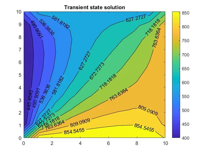

clear all
close all
clc
%Transient state 2d heat conduction equation - Explicit Solution
%(d^2T/dx^2)+(d^2T/dy^2)=(1/alpha)*(dT/dt)

alpha = 1.4; %thermal conductivity
t = linspace(0,30,1500); dt = t(2)-t(1);

nx = 10;%2d space grid
ny = 10;
x = linspace(0,10,nx); dx = x(3)-x(2);
y = linspace(0,10,ny); dy = y(3)-y(2);

%CFL numbers
k1 = (alpha*dt)/(dx^2);%along X
k2 = (alpha*dt)/(dy^2);%along Y

%2d temperature grid
T = temp_matrix(600,900,400,800,nx,ny);%defined function
T_old = T;

for k = 1:length(t)
    for i = 2:nx-1
        for j = 2:ny-1
            H = T_old(i-1,j)-2*T_old(i,j)+T_old(i+1,j); %horizontal computation
            V = T_old(i,j+1)-2*T_old(i,j)+T_old(i,j-1); %vertical computation
            T(i,j) = T_old(i,j)+(k1*H)+(k2*V);
        end
    end
    time = t(k);
    T_old = T;
    figure(1)
    contourf(T,nx,'edgecolor','none')
    set(gca,'YDIR','reverse');
    title_text = sprintf('Time = %d',time);
    title({title_text;'Transient State Heat Conduction-Explicit Solution'});
    pause(0.005);
end
figure(2) 
[X,Y] = meshgrid(x,y);
contourf(X,flipud(Y),T,nx,'ShowText','on'); 
title('Transient state solution');
colorbar;

function solution = temp_matrix(t,b,l,r,nx,ny)
   
    T = 500*ones(ny,nx);
    T(1,2:nx-1) = t;%top
    T(ny,2:nx-1) = b;%bottom
    T(2:ny-1,1) = l;%left
    T(2:ny-1,nx) = r;%right
    T(1,1) = (t+l)/2; T(1,nx) = (t+r)/2; T(ny,1) = (l+b)/2; T(ny,nx) = (b+r)/2;%corners
    
    solution = T;
end

clear all 
close all
clc

%Transient state 2d heat conduction equation using Implicit scheme
%(d^2T/dx^2)+(d^2T/dy^2)=(1/alpha)*(dT/dt)

alpha = 1.4; %thermal conductivity
t = linspace(0,40,4500); dt = t(2)-t(1);

nx = 10;%2d space grid
ny = 10;
x = linspace(0,10,nx); dx = x(3)-x(2);
y = linspace(0,10,ny); dy = y(3)-y(2);

%CFL numbers
k1 = (alpha*dt)/(dx^2);%along X
k2 = (alpha*dt)/(dy^2);%along Y

%2d temperature grid
T = temp_matrix(600,900,400,800,nx,ny);%defined function
T_old = T;
T_prev_dt = T_old;

error = 9e9;
tolerance = 1e-4;
iteration_no = 1;
iter = 2;

%Jacobi Solver
if iter == 1
    for k = 1:length(t) %time loop
        error = 9e9;
        while(error>tolerance) %convergence loop
            for i=2:nx-1  %space loop
                for j=2:ny-1
                    A = 1/(1+(2*k1)+(2*k2));
                    B = A*k1;
                    C = A*k2;
                    H = T_old(i-1,j)+T_old(i+1,j); %horizontal computation
                    V = T_old(i,j+1)+T_old(i,j-1); %vertical computation
                    T(i,j) = A*T_prev_dt(i,j)+B*H+C*V;
                end
            end
            iteration_no = iteration_no+1;
            error = max(max(abs(T_old-T)));
            T_old = T;
        end
        time = t(k);
        T_prev_dt = T;
        [X,Y] = meshgrid(x,y);
        figure(1)
        contourf(T,nx,'edgecolor','none')
        set(gca,'YDIR','reverse');
        title_text = sprintf('Time = %d',time);
        title({title_text;'Transient State Heat Conduction-Implicit Solution'});
        pause(0.005)   
    end
    figure(2) 
    contourf(X,flipud(Y),T,nx,'ShowText','on'); 
    colorbar;
end

%Gauss Siedal Solver
if iter == 2
    for k = 1:length(t) %time loop
        error = 9e9;
        while(error>tolerance) %convergence loop
            for i=2:nx-1  %space loop
                for j=2:ny-1
                    A = 1/(1+(2*k1)+(2*k2));
                    B = A*k1;
                    C = A*k2;
                    H = T(i-1,j)+T_old(i+1,j); %horizontal computation
                    V = T_old(i,j+1)+T(i,j-1); %vertical computation
                    T(i,j) = A*T_prev_dt(i,j)+B*H+C*V;
                end
            end
            iteration_no = iteration_no+1;
            error = max(max(abs(T_old-T)));
            T_old = T;
        end
        time = t(k);
        T_prev_dt = T;
        [X,Y] = meshgrid(x,y);
        figure(1)
        contourf(T,nx,'edgecolor','none')
        set(gca,'YDIR','reverse');
        title_text = sprintf('Time = %d',time);
        title({title_text;'Transient State Heat Conduction-Implicit Solution'});
        pause(0.005)   
    end
    figure(2) 
    contourf(X,flipud(Y),T,nx,'ShowText','on'); 
    colorbar;
end

function solution = temp_matrix(t,b,l,r,nx,ny)
   
    T = 500*ones(ny,nx);
    T(1,2:nx-1) = t;%top
    T(ny,2:nx-1) = b;%bottom
    T(2:ny-1,1) = l;%left
    T(2:ny-1,nx) = r;%right
    T(1,1) = (t+l)/2; T(1,nx) = (t+r)/2; T(ny,1) = (l+b)/2; T(ny,nx) = (b+r)/2;%corners
    
    solution = T;
end

Observations

1. The number of iterations is directly proportional to the grid size.
2. The following trend is observed in the number of iterations : Jacobi > Gauss-Siedal > SOR