Week 7 - Simulation of a 1D Super-sonic nozzle flow simulation using Macormack Method
A steady, isentropic flow through a convergent-divergent nozzle is considered in this problem. The flow at the inlet to the nozzle comes from a reservoir where the pressure and temperature are denoted by p0 and To respectively. The cross-sectional area of the reservoir is large and hence the velocity is very small . Hence, Po and T0 are the stagnation values or total pressure and total temperature, respectively. The flow expands isentropically to supersonic speeds at the nozzle exit, where the exit pressure, temperature, velocity and Mach number are denoted by Pe, Te, Ve and Me, respectively. The flow is locally subsonic in the convergent section of the nozzle, sonic(equal to the local speed of sound) at the throat(minimum area) and supersonic at the divergent section.
NON CONSERVATIVE FORM OF SUPERSONIC ISENTROPIC NOZZLE FLOW USING MACORMACK METHOD
clear all
close all
clc

%Constants
C_no = 0.5;
gamma = 1.4;

%linear grid
n = 31;
x = linspace(0,3,n);
dx = x(2)-x(1);

%Nozzle shape and initial conditions(t=0)
A = 1+2.2*((x-1.5).^2);     %Area profile
rho = 1-0.3146*x;           %Density profile
T = 1-0.2314*x;             %Temperature profile
v = (0.1+1.09*x).*T.^0.5;   %Velocity profile
P = rho.*T;                 %Pressure profile
M = v./(T.^0.5);             %Mach No profile

%Timestep definition
nt = 1400;

for i = 1:length(x)
    dt(i) = 0.5*(dx/(T(i)^0.5 + v(i))); %to compute the local timesteps using CFL condition
end

dt = min(dt); %minimum value of timestep among the given set

%Timeloop
for j = 1:nt

    rho_old = rho;
    v_old = v;
    T_old = T;
    P_old = P;

    %predictor step
    for k = 2:n-1
        dv_dx = (v(k+1)-v(k))/dx;
        drho_dx = (rho(k+1)-rho(k))/dx;
        dT_dx = (T(k+1)-T(k))/dx;
        dlogA_dx = (log(A(k+1))-log(A(k)))/dx;

        %continuity eqn
        drho_dt_p(k) = (-rho(k)*dv_dx)-(rho(k)*v(k)*dlogA_dx)-(v(k)*(drho_dx));

        %momentum eqn
        dv_dt_p(k) = (-v(k)*dv_dx)-(1/gamma)*(dT_dx + (T(k)/rho(k))*drho_dx);

        %energy eqn
        dT_dt_p(k) = (-v(k)*dT_dx)-(gamma-1)*T(k)*(dv_dx + v(k)*dlogA_dx);

        %updated values
        rho(k) = rho(k)+drho_dt_p(k)*dt;
        v(k) = v(k)+dv_dt_p(k)*dt;
        T(k) = T(k)+dT_dt_p(k)*dt;
    end

    %corrector step
    for l = 2:n-1
        dv_dx = (v(l)-v(l-1))/dx;
        drho_dx = (rho(l)-rho(l-1))/dx;
        dT_dx = (T(l)-T(l-1))/dx;
        dlogA_dx = (log(A(l))-log(A(l-1)))/dx;

        %continuity eqn
        drho_dt_c(l) = (-rho(l)*dv_dx)-(rho(l)*v(l)*dlogA_dx)-(v(l)*(drho_dx));

        %momentum eqn
        dv_dt_c(l) = (-v(l)*dv_dx)-(1/gamma)*(dT_dx + (T(l)/rho(l))*drho_dx);

        %energy eqn
        dT_dt_c(l) = (-v(l)*dT_dx)-(gamma-1)*T(l)*(dv_dx + v(l)*dlogA_dx);
    end

    %average values
    drho_dt_avg = 0.5*(drho_dt_p + drho_dt_c);
    dv_dt_avg = 0.5*(dv_dt_p + dv_dt_c);
    dT_dt_avg = 0.5*(dT_dt_p + dT_dt_c);

    %final solution update
    for m = 2:n-1
        rho(m) = rho_old(m)+drho_dt_avg(m)*dt;
        v(m) = v_old(m)+dv_dt_avg(m)*dt;
        T(m) = T_old(m)+dT_dt_avg(m)*dt;
        P(m) = rho(m).*T(m);
        M(m) = v(m)./(T(m).^0.5);
    end

    %boundary conditions
    %inflow
    v(1) = 2*v(2)-v(3);
    %outflow
    v(n) = 2*v(n-1)-v(n-2);
    T(n) = 2*T(n-1)-T(n-2);
    rho(n) = 2*rho(n-1)-rho(n-2);
    P(n) = 2*P(n-1)-P(n-2);
    M(n) = 2*M(n-1)-M(n-2);

%     figure(1)
%     plot(x,v)
%     xlabel('Nozzle length');
%     ylabel('Velocity');
%     title({'Non-Conservative Form',sprintf('Time step =%d',j)})
%     pause(0.03)
%
%     figure(2)
%     plot(x,rho)
%     xlabel('Nozzle length');
%     ylabel('Density');
%     title({'Non-Conservative Form',sprintf('Time step =%d',j)})
%     pause(0.03)
%
%     figure(3)
%     plot(x,T)
%     xlabel('Nozzle length');
%     ylabel('Temperature');
%     title({'Non-Conservative Form',sprintf('Time step =%d',j)})
%     pause(0.03)
%
%     figure(4)
%     plot(x,M)
%     xlabel('Nozzle length');
%     ylabel('Mach No');
%     title({'Non-Conservative Form',sprintf('Time step =%d',j)})
%     pause(0.03)
%
%     figure(5)
%     plot(x,P)
%     xlabel('Nozzle length');
%     ylabel('Pressure');
%     title({'Non-Conservative Form',sprintf('Time step =%d',j)})
%     pause(0.03)

    %Mass Flow Rate variation
    figure(6)
    plot(x,rho.*v.*A)
    axis([0 3 0.4 0.8])
    xlabel('Nozzle length');
    ylabel('Mass Flow Rate');
    title({'Variation of Mass Flow Rate',sprintf('Time step =%d',j)})
    pause(0.03)
end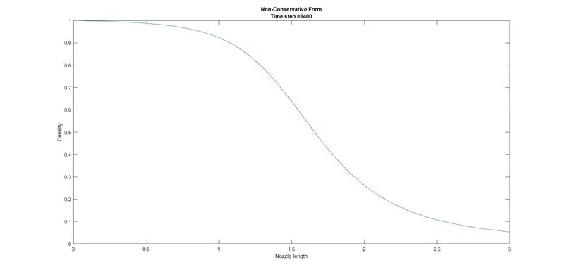
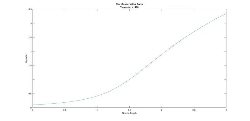
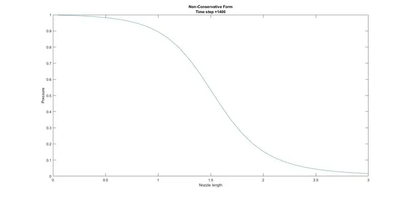
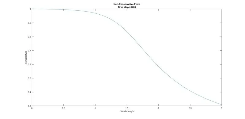
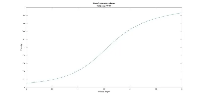
At the subsonic section of the nozzle, the primitive variables such as Density, Pressure and Temperature corresponds to the stagnation values at the inlet and gradually drops in magnitude as the flow approaches the throat of the nozzle. These variables further drop in magnitude as the flow approaches supersonic speeds and exits the nozzle at almost null values. The presence of pressure gradient Po/Pe across the nozzle provides the necessary acceleration to the flow.At the reservoir, the velocity and corresponding Mach No. is minimal and the flow achieves supersonic values at the nozzle exit.
There exists a small percentage of variation between the numerical and analytical values. These inaccuracies are due to possibly 3 reasons
- Inflow boundary condition error
- Truncation errors associated with Grid size
- Effect of Courant No.
The mass flow variation fluctuates erratically around inside the nozzle due to the transient variation of the flow-field variables. After 200 time steps, the mass flow distribution begins to settle down, and after 700 time-steps, the mass flow distribution reduces to straight, horizontal line. It can be inferred that the flow approaches steady state condition after 700 timesteps.
CONSERVATIVE FORM FOR SUPERSONIC ISENTROPIC NOZZLE FLOW USING MACORMACK METHOD
clear all
close all
clc

%Constants
C_no = 0.5;
gamma = 1.4;

%linear grid
n = 31;
x = linspace(0,3,n);
dx = x(2)-x(1);

%Nozzle shape and initial conditions(t=0)
A = 1+2.2*((x-1.5).^2);             %Area profile

for  i = 1:6
    rho_1(i) = 1;
    T_1(i) = 1;
    v_1(i) = 0.59/(rho_1(i)*A(i));
end
for  j = 7:16
    rho_2(j) = 1.0-0.366*(x(j)-0.5);
    T_2(j) = 1.0-0.167*(x(j)-0.5);
    v_2(j) = 0.59/(rho_2(j)*A(j));
end
for  k = 17:31
    rho_3(k) = 0.634-0.3879*(x(k)-1.5);
    T_3(k) = 0.833-0.3507*(x(k)-1.5);
    v_3(k) = 0.59/(rho_3(k)*A(k));
end

rho = [rho_1 rho_2(7:16) rho_3(17:31)];     %Density profile
T = [T_1 T_2(7:16) T_3(17:31)];             %Temperature profile
v = [v_1 v_2(7:16) v_3(17:31)];             %velocity profile
P = rho.*T;                                 %Pressure profile
M = v./(T.^0.5);                            %Mach No profile

%representation of primitive variables in terms of solution vector 'U'
U_1 = rho.*A;
U_2 = rho.*A.*v;
U_3 = U_1.*((T/(gamma-1))+(gamma/2)*(v.^2));

%Timestep definition
nt = 1000;
dt = 0.0267;
t = linspace(0,nt*dt,nt);

%Timeloop
for m = 1:nt

    U_1_old = U_1;
    U_2_old = U_2;
    U_3_old = U_3;

    %pure form of flux variables

    F_1 = U_2;
    F_2 = ((U_2.^2)./U_1)+((gamma-1)/gamma)*(U_3 - ((gamma/2)*((U_2.^2)./U_1)));
    F_3 = ((gamma*(U_2.*U_3))./U_1)-((gamma*(gamma-1)/2)*((U_2.^3)./(U_1.^2)));

    %predictor step
    for o = 2:n-1
        dF_1_dx = (F_1(o+1)-F_1(o))/dx;
        dF_2_dx = (F_2(o+1)-F_2(o))/dx;
        dF_3_dx = (F_3(o+1)-F_3(o))/dx;
        J_2(o) = (1/gamma)*(rho(o)*T(o)).*((A(o+1)-A(o))/dx);

        dU_1_dt_p(o) = -(dF_1_dx);          %continuity eqn
        dU_2_dt_p(o) = -(dF_2_dx)+J_2(o);   %momentum eqn
        dU_3_dt_p(o) = -(dF_3_dx);          %energy eqn

        %updated values
        U_1(o) = U_1(o)+dU_1_dt_p(o)*dt;
        U_2(o) = U_2(o)+dU_2_dt_p(o)*dt;
        U_3(o) = U_3(o)+dU_3_dt_p(o)*dt;

    end

%       rho = U_1./A;
%       v = U_2./U_1;
%       T = (gamma-1)*((U_3./U_1)-((gamma/2)*((U_2./U_1).^2)));

        F_1 = U_2;
        F_2 = ((U_2.^2)./U_1)+((gamma-1)/gamma)*(U_3 - ((gamma/2).*((U_2.^2)./U_1)));
        F_3 = ((gamma*(U_2.*U_3))./U_1)-((gamma*(gamma-1)/2)*((U_2.^3)./(U_1.^2)));

    %corrector step
    for q = 2:n-1
        dF_1_dx = (F_1(q)-F_1(q-1))/dx;
        dF_2_dx = (F_2(q)-F_2(q-1))/dx;
        dF_3_dx = (F_3(q)-F_3(q-1))/dx;
        J_2(q) = (1/gamma)*(rho(q)*T(q)).*((A(q)-A(q-1))/dx);

        dU_1_dt_c(q) = -(dF_1_dx);          %continuity eqn

        dU_2_dt_c(q) =  -(dF_2_dx)+J_2(q);     %momentum eqn

        dU_3_dt_c(q) = -(dF_3_dx);          %energy eqn
    end

    %Average values
    dU_1_dt_avg = 0.5*(dU_1_dt_p + dU_1_dt_c);
    dU_2_dt_avg = 0.5*(dU_2_dt_p + dU_2_dt_c);
    dU_3_dt_avg = 0.5*(dU_3_dt_p + dU_3_dt_c);

    %final solution update
    for r = 2:n-1
        U_1(r) = U_1_old(r)+dU_1_dt_avg(r)*dt;
        U_2(r) = U_2_old(r)+dU_2_dt_avg(r)*dt;
        U_3(r) = U_3_old(r)+dU_3_dt_avg(r)*dt;
    end

    %boundary conditions
    %inflow
    U_1(1) = A(1);
    U_2(1) = 2*U_2(2)-U_2(3);
    U_3(1) = U_1(1)*((T(1)/(gamma-1))+(gamma/2)*(((U_2(1)/U_1(1))^2)));

    %outflow
    U_1(n) = 2*U_1(n-1)-U_1(n-2);
    U_2(n) = 2*U_2(n-1)-U_2(n-2);
    U_3(n) = 2*U_3(n-1)-U_3(n-2);

    rho = U_1./A;
    v = U_2./U_1;
    T = (gamma-1)*((U_3./U_1)-((gamma/2)*(v.^2)));
    P = rho.*T;
    M = v./(T.^0.5);

    figure(1)
    plot(x,v)
    xlabel('Nozzle length');
    ylabel('Velocity');
    title({'Conservative Form',sprintf('Time step =%d',m)})
    pause(0.03)

    figure(2)
    plot(x,rho)
    xlabel('Nozzle length');
    ylabel('Density');
    title({'Conservative Form',sprintf('Time step =%d',m)})
    pause(0.03)

    figure(3)
    plot(x,T)
    xlabel('Nozzle length');
    ylabel('Temperature');
    title({'Conservative Form',sprintf('Time step =%d',m)})
    pause(0.03)

    figure(4)
    plot(x,M)
    xlabel('Nozzle length');
    ylabel('Mach No');
    title({'Conservative Form',sprintf('Time step =%d',m)})
    pause(0.03)

    figure(5)
    plot(x,P)
    xlabel('Nozzle length');
    ylabel('Pressure');
    title({'Conservative Form',sprintf('Time step =%d',m)})
    pause(0.03)

%Mass Flow Rate variation
    figure(6)
    plot(x,rho.*v.*A)
    axis([0 3 0.4 0.8])
    xlabel('Nozzle length');
    ylabel('Mass Flow Rate');
    title({'Variation of Mass Flow Rate',sprintf('Time step =%d',m)})
    pause(0.03)
end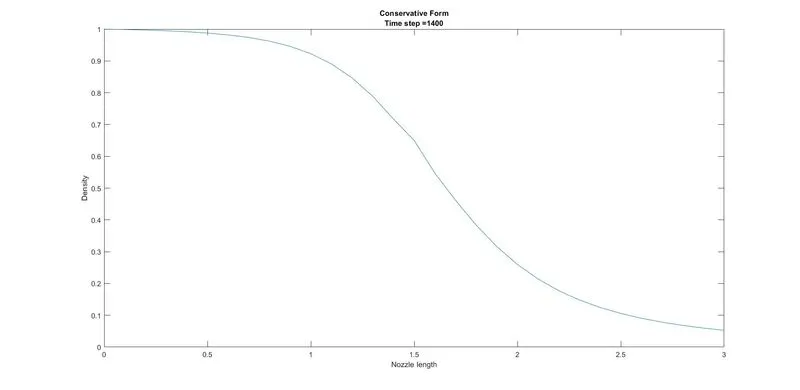
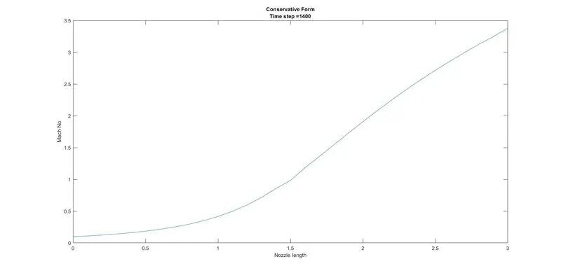
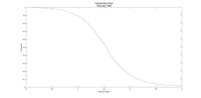
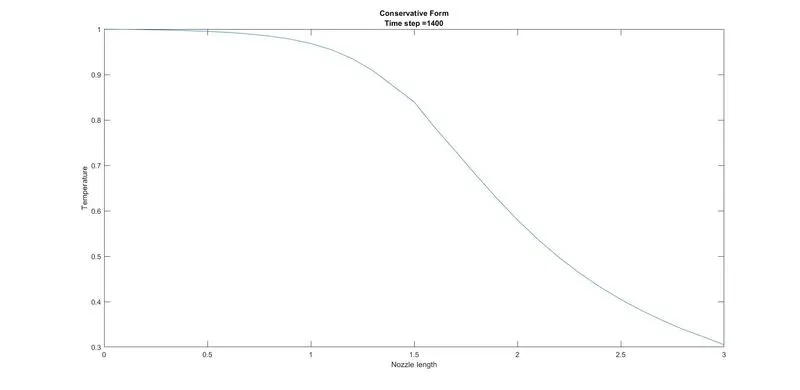
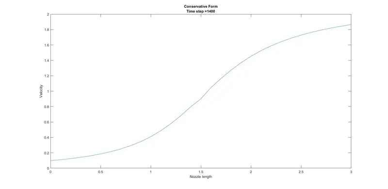
The steady-state results obtained from the time-marching solution of the governing equations in conservation form are essentially the same as those obtained using the non-conservation form. A quick comparison of both forms show little difference and hence it can be concluded that, for all practical purposes, both forms of the governing equations give the same results. One notable difference is in the mass flow distribution. At steady state, the conservative form of governing equations exhibits a mass flow with minimal variation in magnitude across the nozzle length and also the values of mass flow are closer to the exact analytical solution. In contrast, the non-conservative form produces mass flow values which have relatively large fluctuation from the mean value at the inlet and outlet and also slightly more deviated from the exact solution as compared to the difference between conservative form value and exact solution.
The non-conservative form produces slightly more accurate results for the primitive variables, and the conservation form seems to produce slightly more accurate results for the flux variables.
The conservative form requires decoding the primitive variables from the flux variables and hence there is more effort involved. On the other hand, the non-conservative form does not involve this process.