Week 12 - Validation studies of Symmetry BC vs Wedge BC in OpenFOAM vs Analytical H.P equation
Objective - To simulate an axisymmetric flow by applying the wedge (for wedge angle of 3°,4° and 5°) and symmetry (for wedge angle of 10°,25° and 45°) boundary conditions using Matlab and OpenFOAM. The working fluid is assumed to be water at 25°C and flow is laminar and it flows through a constant cross-section pipe at an inlet Reynold's number of 2100. The results of the simulation are compared with each other and validated with the Hagen- Poiseuille's equations for the fully developed flow.
Methodology - An angular block/section of the circular pipe with angles of 3°,4°,5°,10°,25° and 45° are studied assuming the flow parameters with respect to angle does not vary. The blockMeshDict files for wedge and symmetry boundary conditions are created using Matlab. To simulate an incompressible laminar flow case, the icoFoam solver is used in OpenFOAM after the necessary changes are made to the initial conditions(p and U) and the controlDict file with reference to newly created blockMeshDict file using Matlab. Paraview is used to post-process the results once the simulation is complete.
Matlab code to generate blockMeshDict file with symmetry boundary condition
 clear all
 close all
 clc

 % Defining the variables
 Re = 2100;        %Reynolds Number
 D = 0.005;        %Diameter of pipe (m)
 L = 0.06*Re*D;    %Entry length of pipe (m)
 L_full = L+0.87;   %Total length of pipe (m)
 r = D/2;          %Radius of pipe (m)
 theta = 10;        %Wedge Angle (less than 5 deg)
 mu = 0.8891e-3;   %Dynamic viscosity @ 25 deg (Ns/m^2)
 rho = 997;        %Density (kg/m^3)
 nu = mu/rho;      %Kinematic viscosity @ 25 deg (m^2/s)

 %variables from Hagen-Poiseuille Equation
 v_avg = (Re*mu)/(rho*D);
 v_max = 2*(v_avg);
 del_p = (8*mu*L_full*v_avg)/(r^2);
 kinematic_p = del_p/rho;
 head_loss = del_p/(9.81*rho);

 h1 = '/*--------------------------------*- C++ -*----------------------------------*\';
 h2 = '  =========                 |                                                  ';
 h3 = '  \\      /  F ield         | OpenFOAM: The Open Source CFD Toolbox            ';
 h4 = '   \\    /   O peration     | Website:  https://openfoam.org                   ';
 h5 = '    \\  /    A nd           | Version:  8                                      ';
 h6 = '     \\/     M anipulation  |                                                  ';
 h7 = '\*---------------------------------------------------------------------------*/';
 h8 = '// * * * * * * * * * * * * * * * * * * * * * * * * * * * * * * * * * * * * * //';
 h9 = '// ************************************************************************* //';

 f1 = fopen('blockMeshDict','w');
 fprintf(f1, '%s\n', h1);
 fprintf(f1, '%s\n', h2);
 fprintf(f1, '%s\n', h3);
 fprintf(f1, '%s\n', h4);
 fprintf(f1, '%s\n', h5);
 fprintf(f1, '%s\n', h6);
 fprintf(f1, '%s\n', h7);

 fprintf(f1, 'FoamFile\n{\n');
 fprintf(f1, '%12s \t 2.0;\n','version');
 fprintf(f1, '%12s \t ascii;\n','format');
 fprintf(f1, '%12s \t dictionary;\n','class');
 fprintf(f1, '%12s \t blockMeshDict;\n','object');
 fprintf(f1, '}\n');
 fprintf(f1, '%s\n\n',h8);


 fprintf(f1, 'convertToMeters 1;\n\n');

 fprintf(f1, 'vertices\n');
 fprintf(f1, '(\n');
 fprintf(f1, '\t (%d %d %d)\n',0,0,0);
 fprintf(f1, '\t (%d %d %d)\n',0,r*cosd(theta/2),r*sind(theta/2));
 fprintf(f1, '\t (%d %d %d)\n',0,r*cosd(theta/2),-r*sind(theta/2));
 fprintf(f1, '\t (%d %d %d)\n',L_full,0,0);
 fprintf(f1, '\t (%d %d %d)\n',L_full,r*cosd(theta/2),r*sind(theta/2));
 fprintf(f1, '\t (%d %d %d)\n',L_full,r*cosd(theta/2),-r*sind(theta/2));
 fprintf(f1, ');\n\n');


 fprintf(f1, 'blocks\n');
 fprintf(f1, '(\n');
 fprintf(f1, '\t hex (0 3 5 2 0 3 4 1) (%d %d %d)',500,50,1);
 fprintf(f1, ' SimpleGrading (1 0.1 1)\n\n');
 fprintf(f1, ');\n\n');

 fprintf(f1, 'edges\n');
 fprintf(f1, '(\n');
 fprintf(f1, '\t arc %d %d (%d %d %d)\n',1,2,0,r,0);
 fprintf(f1, '\t arc %d %d (%d %d %d)\n',4,5,L_full,r,0);
 fprintf(f1, ');\n\n');

 fprintf(f1, 'boundary\n');
 fprintf(f1, '(\n');
 fprintf(f1, '\t inlet \n');
 fprintf(f1, '\t {\n');
 fprintf(f1, '\t\t type patch;\n');
 fprintf(f1, '\t\t faces\n');
 fprintf(f1, '\t\t (\n');
 fprintf(f1, '\t\t\t (0 1 2 0)\n');
 fprintf(f1, '\t\t );\n');
 fprintf(f1, '\t }\n');


 fprintf(f1, '\t outlet\n');
 fprintf(f1, '\t {\n');
 fprintf(f1, '\t\t type patch;\n');
 fprintf(f1, '\t\t faces\n');
 fprintf(f1, '\t\t (\n');
 fprintf(f1, '\t\t\t (3 5 4 3)\n');
 fprintf(f1, '\t\t );\n');
 fprintf(f1, '\t }\n');


 fprintf(f1, '\t top\n');
 fprintf(f1, '\t {\n');
 fprintf(f1, '\t\t type wall;\n');
 fprintf(f1, '\t\t faces\n') ;
 fprintf(f1, '\t\t (\n');
 fprintf(f1, '\t\t\t (1 4 5 2)\n');
 fprintf(f1, '\t\t );\n');
 fprintf(f1, '\t }\n');

 fprintf(f1, '\t front\n');
 fprintf(f1, '\t {\n');
 fprintf(f1, '\t\t type symmetry;\n');
 fprintf(f1, '\t\t faces\n');
 fprintf(f1, '\t\t (\n');
 fprintf(f1, '\t\t\t (0 3 4 1)\n');
 fprintf(f1, '\t\t );\n');
 fprintf(f1, '\t }\n');

 fprintf(f1, '\t back\n');
 fprintf(f1, '\t {\n');
 fprintf(f1, '\t\t type symmetry;\n');
 fprintf(f1, '\t\t faces\n');
 fprintf(f1, '\t\t (\n');
 fprintf(f1, '\t\t\t (0 2 5 3)\n');
 fprintf(f1, '\t\t );\n');
 fprintf(f1, '\t }\n');

 fprintf(f1, '\t axis\n');
 fprintf(f1, '\t {\n');
 fprintf(f1, '\t\t type empty;\n');
 fprintf(f1, '\t\t faces\n');
 fprintf(f1, '\t\t (\n');
 fprintf(f1, '\t\t\t (0 3 3 0)\n');
 fprintf(f1, '\t\t );\n');
 fprintf(f1, '\t }\n');
 fprintf(f1, '); \n\n');

 fprintf(f1, 'mergePatchPairs\n');
 fprintf(f1, '(\n');
 fprintf(f1, ');\n');

 fprintf(f1, '%s\n',h9);

 fclose(f1);
Output blockMeshDict file
/*--------------------------------*- C++ -*----------------------------------*\
  =========                 |
  \\      /  F ield         | OpenFOAM: The Open Source CFD Toolbox
   \\    /   O peration     | Website:  https://openfoam.org
    \\  /    A nd           | Version:  8
     \\/     M anipulation  |
\*---------------------------------------------------------------------------*/
FoamFile
{
     version 	 2.0;
      format 	 ascii;
       class 	 dictionary;
      object 	 blockMeshDict;
}
// * * * * * * * * * * * * * * * * * * * * * * * * * * * * * * * * * * * * * //

convertToMeters 1;

vertices
(
	 (0 0 0)
	 (0 2.490487e-03 2.178894e-04)
	 (0 2.490487e-03 -2.178894e-04)
	 (1.500000e+00 0 0)
	 (1.500000e+00 2.490487e-03 2.178894e-04)
	 (1.500000e+00 2.490487e-03 -2.178894e-04)
);

blocks
(
	 hex (0 3 5 2 0 3 4 1) (1500 150 1) SimpleGrading (1 0.1 1)

);

edges
(
	 arc 1 2 (0 2.500000e-03 0)
	 arc 4 5 (1.500000e+00 2.500000e-03 0)
);

boundary
(
	 inlet
	 {
		 type patch;
		 faces
		 (
			 (0 1 2 0)
		 );
	 }
	 outlet
	 {
		 type patch;
		 faces
		 (
			 (3 5 4 3)
		 );
	 }
	 top
	 {
		 type wall;
		 faces
		 (
			 (1 4 5 2)
		 );
	 }
	 front
	 {
		 type symmetry;
		 faces
		 (
			 (0 3 4 1)
		 );
	 }
	 back
	 {
		 type symmetry;
		 faces
		 (
			 (0 2 5 3)
		 );
	 }
	 axis
	 {
		 type empty;
		 faces
		 (
			 (0 3 3 0)
		 );
	 }
);

mergePatchPairs
(
);
// ************************************************************************* //
The respective controlDict and initial conditions of p and U with modifications in boundary conditions is given
/*--------------------------------*- C++ -*----------------------------------*\
  =========                 |
  \\      /  F ield         | OpenFOAM: The Open Source CFD Toolbox
   \\    /   O peration     | Website:  https://openfoam.org
    \\  /    A nd           | Version:  8
     \\/     M anipulation  |
\*---------------------------------------------------------------------------*/
FoamFile
{
    version     2.0;
    format      ascii;
    class       dictionary;
    location    "system";
    object      controlDict;
}
// * * * * * * * * * * * * * * * * * * * * * * * * * * * * * * * * * * * * * //

application     icoFoam;

startFrom       startTime;

startTime       0;

stopAt          endTime;

endTime         1;

deltaT          0.005;

writeControl    timeStep;

writeInterval   20;

purgeWrite      0;

writeFormat     ascii;

writePrecision  6;

writeCompression off;

timeFormat      general;

timePrecision   6;

runTimeModifiable true;


// ************************************************************************* //
/*--------------------------------*- C++ -*----------------------------------*\
  =========                 |
  \\      /  F ield         | OpenFOAM: The Open Source CFD Toolbox
   \\    /   O peration     | Website:  https://openfoam.org
    \\  /    A nd           | Version:  8
     \\/     M anipulation  |
\*---------------------------------------------------------------------------*/
FoamFile
{
    version     2.0;
    format      ascii;
    class       volScalarField;
    object      p;
}
// * * * * * * * * * * * * * * * * * * * * * * * * * * * * * * * * * * * * * //

dimensions      [0 2 -2 0 0 0 0];

internalField   uniform 0;

boundaryField
{
    inlet
    {
        type            zeroGradient;
    }

    outlet
    {
        type            fixedValue;
        value uniform   0.6413;
    }

    axis
    {
        type            empty;
    }

    top
    {
        type            zeroGradient;
    }

    front
    {
        type            symmetry;
    }

    back
    {
        type            symmetry;
    }
}

// ************************************************************************* //
/*--------------------------------*- C++ -*----------------------------------*\
  =========                 |
  \\      /  F ield         | OpenFOAM: The Open Source CFD Toolbox
   \\    /   O peration     | Website:  https://openfoam.org
    \\  /    A nd           | Version:  8
     \\/     M anipulation  |
\*---------------------------------------------------------------------------*/
FoamFile
{
    version     2.0;
    format      ascii;
    class       volVectorField;
    object      U;
}
// * * * * * * * * * * * * * * * * * * * * * * * * * * * * * * * * * * * * * //

dimensions      [0 1 -1 0 0 0 0];

internalField   uniform (0.3745 0 0);

boundaryField
{
    inlet
    {
        type            fixedValue;
        value           uniform (0.3745 0 0);
    }

    outlet
    {
        type            zeroGradient;
    }

    axis
    {
        type            empty;
    }

    top
    {
        type            noSlip;
    }

    front
    {
        type            symmetry;
    }

    back
    {
        type            symmetry;
    }
}

// ************************************************************************* //
The above mentioned codes are similar for other wedge angles of 25° and 45° with the necessary changes in the value of theta variable.
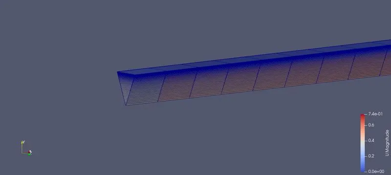
Image showing meshed geometry wegde angle of 45° with symmetry BC
Results and Observation
A matlab is written as shown below to compare the velocity, shear stress and pressure drop of various cases in the simulation with wedge and symmetry BC to the analytical solution as given by HP equations.
clear all
close all
clc

%Analytical velocity of fully developed flow
mu = 0.8891e-3;
U_avg = 0.3745;
r_max = 0.0025;
r = linspace(0,r_max,1001);

for i = 1:length(r)
    V_analytical(i) = 2*U_avg*(1-((r(i)^2)/(r_max^2)));
end

%Parsing Simulated data of fully developed velocity profile from Paraview.
f1 = fopen('veldata_w3.txt','r');
fgetl(f1);
A = fscanf(f1, '%f');
V_1 = A(1:2:end);
V_w3 = V_1';
R = A(2:2:end);
r_1 = R';

f2 = fopen('veldata_w4.txt','r');
fgetl(f2);
B = fscanf(f2, '%f');
V_2 = B(1:2:end);
V_w4 = V_2';

f3 = fopen('veldata_w5.txt','r');
fgetl(f3);
C = fscanf(f3, '%f');
V_3 = C(1:2:end);
V_w5 = V_3';

f4 = fopen('veldata_s10.txt','r');
fgetl(f4);
D = fscanf(f4, '%f');
V_4 = D(1:2:end);
V_s10 = V_4';

f5 = fopen('veldata_s25.txt','r');
fgetl(f5);
E = fscanf(f5, '%f');
V_5 = E(1:2:end);
V_s25 = V_5';

f6 = fopen('veldata_s45.txt','r');
fgetl(f6);
F = fscanf(f6, '%f');
V_6 = F(1:2:end);
V_s45 = V_6';

%plot to validate simulated to anaytical velocity data
figure(1)
plot(V_analytical,r,'k')
hold on
plot(V_w3, r_1,'r')
hold on
plot(V_w4, r_1,'g')
hold on
plot(V_w5, r_1,'b')
hold on
plot(V_s10, r_1,'c')
hold on
plot(V_s25, r_1,'m')
hold on
plot(V_s45, r_1,'y')
hold on
plot(V_analytical,-r,'k')
hold on
plot(V_w3,-r_1,'r')
hold on
plot(V_w4,-r_1,'g')
hold on
plot(V_w5,-r_1,'b')
hold on
plot(V_s10,-r_1,'c')
hold on
plot(V_s25,-r_1,'m')
hold on
plot(V_s45,-r_1,'y')
hold off
grid
title('Velocity profile of fully developed flow');
legend('Analytical','wedge 3','wedge 4','wedge 5','symmetry 10','symmetry 25','symmetry 45')
xlabel('Velocity (m/s)')
ylabel('Diameter (m)')

%Shear stress
for j = 2:length(r)
    Tau_analytical(j) = mu*((V_analytical(j-1)-V_analytical(j))/(r(j)-r(j-1)));
    Tau_w3(j) = mu*((V_w3(j-1)-V_w3(j))/(r(j)-r(j-1)));
    Tau_w4(j) = mu*((V_w4(j-1)-V_w4(j))/(r(j)-r(j-1)));
    Tau_w5(j) = mu*((V_w5(j-1)-V_w5(j))/(r(j)-r(j-1)));
    Tau_s10(j) = mu*((V_s10(j-1)-V_s10(j))/(r(j)-r(j-1)));
    Tau_s25(j) = mu*((V_s25(j-1)-V_s25(j))/(r(j)-r(j-1)));
    Tau_s45(j) = mu*((V_s45(j-1)-V_s45(j))/(r(j)-r(j-1)));
end

figure(2)
plot(Tau_analytical,r,'k')
hold on
plot(Tau_w3,r,'r')
hold on
plot(Tau_w4,r,'g')
hold on
plot(Tau_w5,r,'b')
hold on
plot(Tau_s10,r,'c')
hold on
plot(Tau_s25,r,'m')
hold on
plot(Tau_s45,r,'y')
hold on
plot(Tau_analytical,-r,'k')
hold on
plot(Tau_w3,-r,'r')
hold on
plot(Tau_w4,-r,'g')
hold on
plot(Tau_w5,-r,'b')
hold on
plot(Tau_s10,-r,'c')
hold on
plot(Tau_s25,-r,'m')
hold on
plot(Tau_s45,-r,'y')
hold off
grid
title('Shear stress of fully developed flow');
legend('Analytical','wedge 3','wedge 4','wedge 5','symmetry 10','symmetry 25','symmetry 45')
xlabel('Shear Stress (Pa)')
ylabel('Diameter (m)')

%Pressure drop
f7 = fopen('pressuredata_w3.txt','r');
fgetl(f7);
F = fscanf(f7, '%f');
P_1 = F(1:2:end);
p_w3 = P_1';
l = F(2:2:end);
L = l';

f8 = fopen('pressuredata_w4.txt','r');
fgetl(f8);
G = fscanf(f8, '%f');
P_2 = G(1:2:end);
p_w4 = P_2';

f9 = fopen('pressuredata_w5.txt','r');
fgetl(f9);
H = fscanf(f9, '%f');
P_3 = H(1:2:end);
p_w5 = P_3';

f10 = fopen('pressuredata_s10.txt','r');
fgetl(f10);
I = fscanf(f10, '%f');
P_4 = I(1:2:end);
p_s10 = P_4';

f11 = fopen('pressuredata_s25.txt','r');
fgetl(f11);
J = fscanf(f11, '%f');
P_5 = J(1:2:end);
p_s25 = P_5';

f12 = fopen('pressuredata_s45.txt','r');
fgetl(f12);
K = fscanf(f12, '%f');
P_6 = K(1:2:end);
p_s45 = P_6';

figure(3)
plot(p_w3,L,'k')
hold on
plot(p_w4,L,'r')
hold on
plot(p_w5,L,'g')
hold on
plot(p_s10,L,'b')
hold on
plot(p_s25,L,'c')
hold on
plot(p_s45,L,'m')
hold off
grid
title('Pressure drop across length of pipe');
legend('wedge 3','wedge 4','wedge 5','symmetry 10','symmetry 25','symmetry 45')
xlabel('Pressure drop(Pa)')
ylabel('Length(m)')
Comparison between analytical( Hagen - Poiseulle equations) and simulated results
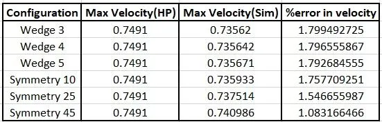
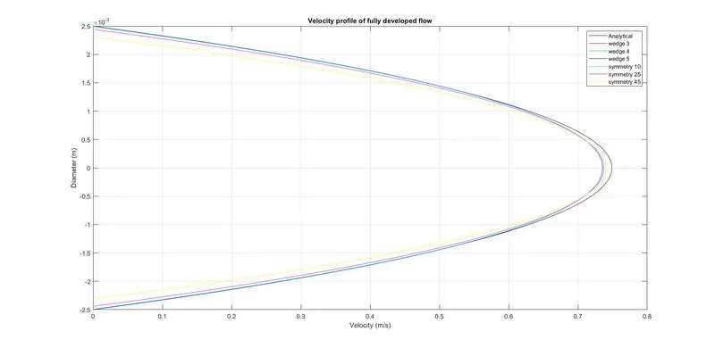
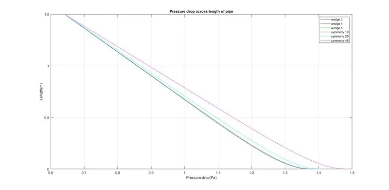
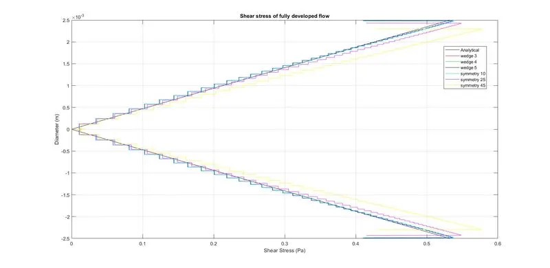
The symmetry BC enables the domain to be halved, reducing the time to achieve a solution and also as seen from the results, it generates a solution with lesser error in comparison with wedge boundary condition. The wedge BC is used in computational fluid dynamics to define an axisymmetric case. The model and flow must be axisymmetric along a central line such that all physical variables of the flow have the same value and distribution at a given radius for all angles. The most ideal case to be in close correlation with the analytical solution is the case with wedge of 45° and symmetry boundary condition.