Week 11 - Simulation of Flow through a pipe in OpenFoam
Objective - To simulate an axisymmetric flow by applying the wedge boundary condition using Matlab and OpenFOAM. The working fluid is assumed to be water at 25°C and flow is laminar and it flows through a constant cross-section pipe at an inlet Reynold's number of 2100. The results of the simulation are validated with the Hagen- Poiseuille's equations for the fully developed flow.
Introduction
1. Reynold's Number
The flow regime depends mainly on the ratio of inertial forces to viscous forces in the fluid and this ratio is called the Reynolds number and is expressed for internal flow in a circular pipe as
`Re = (underset(avg)(V).D)/nu = (rho.underset(avg)(V).D)/mu`
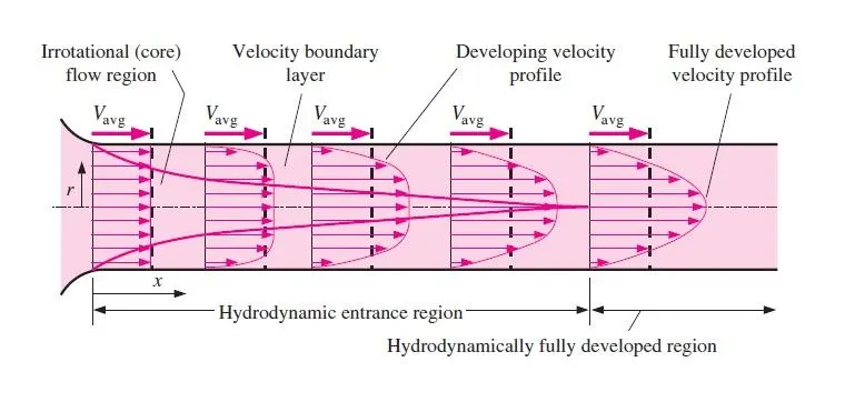
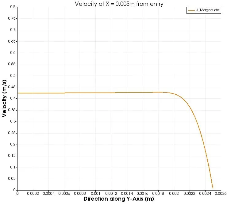
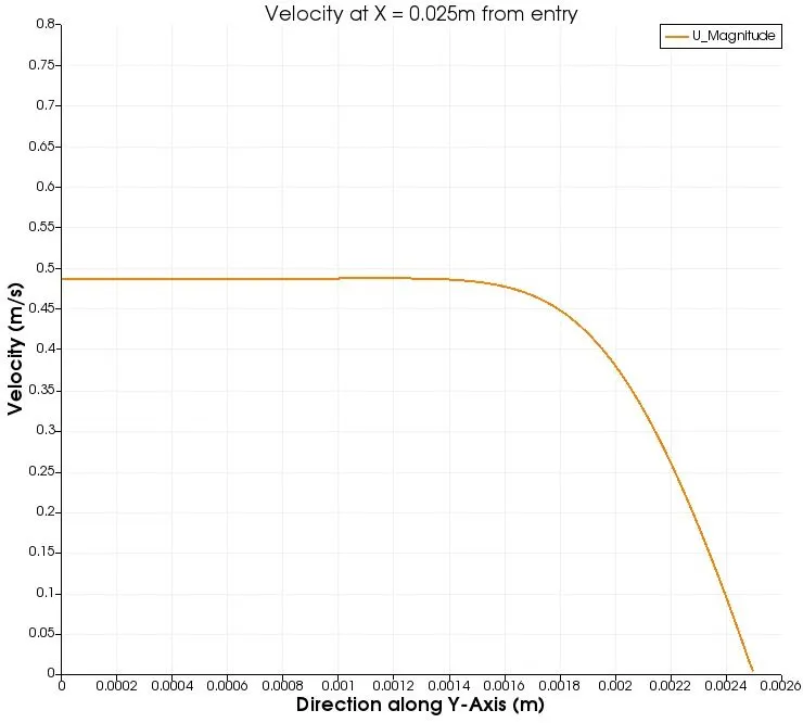
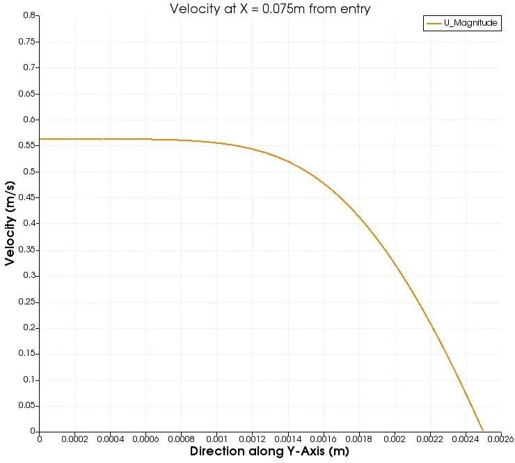
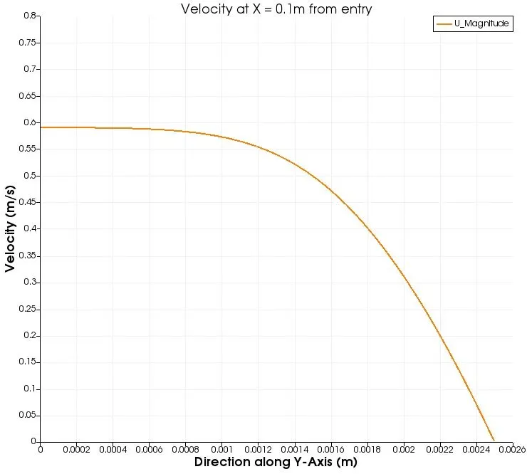
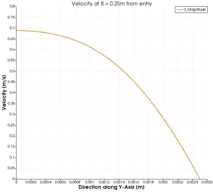
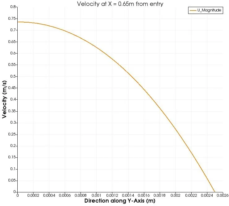
2. A fluid entering a circular pipe at a uniform velocity experiences a no-slip condition as a result the fluid particles in the layer in contact with the surface of the pipe come to a complete stop. This layer also causes the fluid particles in the adjacent layers to slow down gradually as a result of friction. To make up for this velocity reduction, the velocity of the fluid at the midsection of the pipe has to increase to keep the mass flow rate through the pipe constant. As a result, a velocity gradient develops along the pipe which forms a boundary layer. The thickness of this boundary layer increases in the flow direction until the boundary layer reaches the pipe center and thus fills the entire pipe. The region from the pipe inlet to the point at which the boundary layer merges at the centerline is called the hydrodynamic entry length Lh. Flow in the entrance region is called hydrodynamically developing flow since this is the region where the velocity profile develops. The region beyond the entrance region in which the velocity profile is fully developed and remains unchanged is called the hydrodynamically fully developed region. The flow is said to be fully developed when the normalized temperature profile remains unchanged as well.
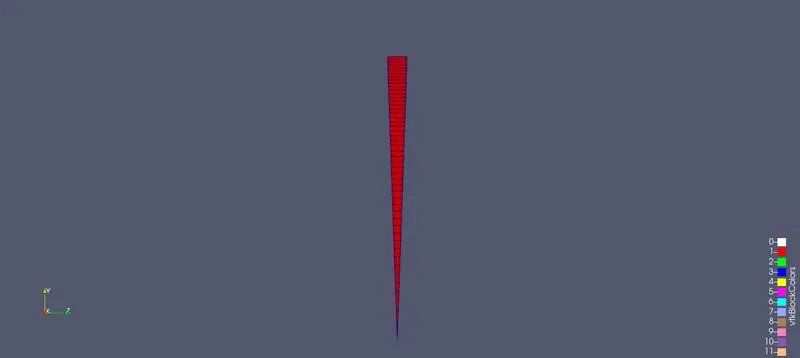
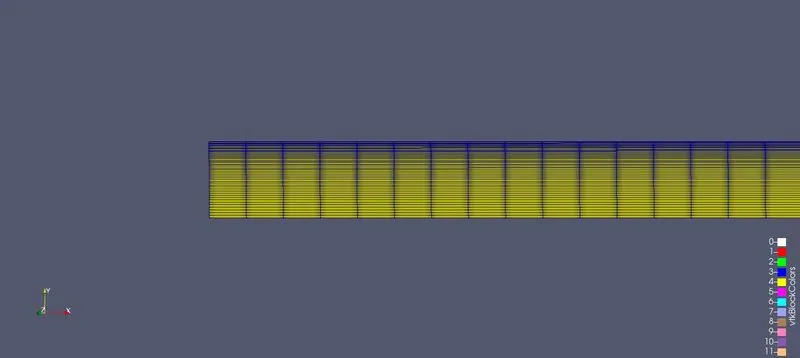
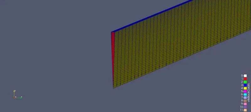
Methodology - An angular block/section of the circular pipe with angle less 5° is studied assuming the flow parameters with respect to angle does not vary. The blockMeshDict file is created using Matlab as shown. To simulate an incompressible laminar flow case, the icoFoam solver is used in OpenFOAM after the necessary changes are made to the initial conditions(p and U) and the controlDict file with reference to newly created blockMeshDict file using Matlab. Paraview is used to post-process the results once the simulation is complete.
Matlab code to generate blockMeshDict file
 clear all
 close all
 clc

 % Defining the variables
 Re = 2100;        %Reynolds Number
 D = 0.005;        %Diameter of pipe (m)
 L = 0.06*Re*D;    %Entry length of pipe (m)
 L_full = L+0.87;  %Total length of pipe (m)
 r = D/2;          %Radius of pipe (m)
 theta = 4;        %Wedge Angle (less than 5 deg)
 mu = 0.8891e-3;   %Dynamic viscosity @ 25 deg (Ns/m^2)
 rho = 997;        %Density (kg/m^3)
 nu = mu/rho;      %Kinematic viscosity @ 25 deg (m^2/s)

 %variables from Hagen-Poiseuille Equation
 v_avg = (Re*mu)/(rho*D);
 v_max = 2*(v_avg);
 del_p = (8*mu*L_full*v_avg)/(r^2);
 kinematic_p = del_p/rho;
 head_loss = del_p/(9.81*rho);

 h1 = '/*--------------------------------*- C++ -*----------------------------------*\';
 h2 = '  =========                 |                                                  ';
 h3 = '  \\      /  F ield         | OpenFOAM: The Open Source CFD Toolbox            ';
 h4 = '   \\    /   O peration     | Website:  https://openfoam.org                   ';
 h5 = '    \\  /    A nd           | Version:  8                                      ';
 h6 = '     \\/     M anipulation  |                                                  ';
 h7 = '\*---------------------------------------------------------------------------*/';
 h8 = '// * * * * * * * * * * * * * * * * * * * * * * * * * * * * * * * * * * * * * //';
 h9 = '// ************************************************************************* //';

 f1 = fopen('blockMeshDict','w');
 fprintf(f1, '%s\n', h1);
 fprintf(f1, '%s\n', h2);
 fprintf(f1, '%s\n', h3);
 fprintf(f1, '%s\n', h4);
 fprintf(f1, '%s\n', h5);
 fprintf(f1, '%s\n', h6);
 fprintf(f1, '%s\n', h7);

 fprintf(f1, 'FoamFile\n{\n');
 fprintf(f1, '%12s \t 2.0;\n','version');
 fprintf(f1, '%12s \t ascii;\n','format');
 fprintf(f1, '%12s \t dictionary;\n','class');
 fprintf(f1, '%12s \t blockMeshDict;\n','object');
 fprintf(f1, '}\n');
 fprintf(f1, '%s\n\n',h8);


 fprintf(f1, 'convertToMeters 1;\n\n');

 fprintf(f1, 'vertices\n');
 fprintf(f1, '(\n');
 fprintf(f1, '\t (%d %d %d)\n',0,0,0);
 fprintf(f1, '\t (%d %d %d)\n',0,r*cosd(theta/2),r*sind(theta/2));
 fprintf(f1, '\t (%d %d %d)\n',0,r*cosd(theta/2),-r*sind(theta/2));
 fprintf(f1, '\t (%d %d %d)\n',L_full,0,0);
 fprintf(f1, '\t (%d %d %d)\n',L_full,r*cosd(theta/2),r*sind(theta/2));
 fprintf(f1, '\t (%d %d %d)\n',L_full,r*cosd(theta/2),-r*sind(theta/2));
 fprintf(f1, ');\n\n');


 fprintf(f1, 'blocks\n');
 fprintf(f1, '(\n');
 fprintf(f1, '\t hex (0 3 5 2 0 3 4 1) (%d %d %d)',500,50,1);
 fprintf(f1, ' SimpleGrading (1 0.1 1)\n\n');
 fprintf(f1, ');\n\n');

 fprintf(f1, 'edges\n');
 fprintf(f1, '(\n');
 fprintf(f1, '\t arc %d %d (%d %d %d)\n',1,2,0,r,0);
 fprintf(f1, '\t arc %d %d (%d %d %d)\n',4,5,L_full,r,0);
 fprintf(f1, ');\n\n');

 fprintf(f1, 'boundary\n');
 fprintf(f1, '(\n');
 fprintf(f1, '\t inlet \n');
 fprintf(f1, '\t {\n');
 fprintf(f1, '\t\t type patch;\n');
 fprintf(f1, '\t\t faces\n');
 fprintf(f1, '\t\t (\n');
 fprintf(f1, '\t\t\t (0 1 2 0)\n');
 fprintf(f1, '\t\t );\n');
 fprintf(f1, '\t }\n');


 fprintf(f1, '\t outlet\n');
 fprintf(f1, '\t {\n');
 fprintf(f1, '\t\t type patch;\n');
 fprintf(f1, '\t\t faces\n');
 fprintf(f1, '\t\t (\n');
 fprintf(f1, '\t\t\t (3 5 4 3)\n');
 fprintf(f1, '\t\t );\n');
 fprintf(f1, '\t }\n');


 fprintf(f1, '\t top\n');
 fprintf(f1, '\t {\n');
 fprintf(f1, '\t\t type wall;\n');
 fprintf(f1, '\t\t faces\n') ;
 fprintf(f1, '\t\t (\n');
 fprintf(f1, '\t\t\t (1 4 5 2)\n');
 fprintf(f1, '\t\t );\n');
 fprintf(f1, '\t }\n');

 fprintf(f1, '\t front\n');
 fprintf(f1, '\t {\n');
 fprintf(f1, '\t\t type wedge;\n');
 fprintf(f1, '\t\t faces\n');
 fprintf(f1, '\t\t (\n');
 fprintf(f1, '\t\t\t (0 3 4 1)\n');
 fprintf(f1, '\t\t );\n');
 fprintf(f1, '\t }\n');

 fprintf(f1, '\t back\n');
 fprintf(f1, '\t {\n');
 fprintf(f1, '\t\t type wedge;\n');
 fprintf(f1, '\t\t faces\n');
 fprintf(f1, '\t\t (\n');
 fprintf(f1, '\t\t\t (0 2 5 3)\n');
 fprintf(f1, '\t\t );\n');
 fprintf(f1, '\t }\n');

 fprintf(f1, '\t axis\n');
 fprintf(f1, '\t {\n');
 fprintf(f1, '\t\t type empty;\n');
 fprintf(f1, '\t\t faces\n');
 fprintf(f1, '\t\t (\n');
 fprintf(f1, '\t\t\t (0 3 3 0)\n');
 fprintf(f1, '\t\t );\n');
 fprintf(f1, '\t }\n');
 fprintf(f1, '); \n\n');

 fprintf(f1, 'mergePatchPairs\n');
 fprintf(f1, '(\n');
 fprintf(f1, ');\n');

 fprintf(f1, '%s\n',h9);

 fclose(f1);
Output blockMeshDict file
/*--------------------------------*- C++ -*----------------------------------*\
  =========                 |
  \\      /  F ield         | OpenFOAM: The Open Source CFD Toolbox
   \\    /   O peration     | Website:  https://openfoam.org
    \\  /    A nd           | Version:  8
     \\/     M anipulation  |
\*---------------------------------------------------------------------------*/
FoamFile
{
     version 	 2.0;
      format 	 ascii;
       class 	 dictionary;
      object 	 blockMeshDict;
}
// * * * * * * * * * * * * * * * * * * * * * * * * * * * * * * * * * * * * * //

convertToMeters 1;

vertices
(
	 (0 0 0)
	 (0 2.498477e-03 8.724874e-05)
	 (0 2.498477e-03 -8.724874e-05)
	 (1.500000e+00 0 0)
	 (1.500000e+00 2.498477e-03 8.724874e-05)
	 (1.500000e+00 2.498477e-03 -8.724874e-05)
);

blocks
(
	 hex (0 3 5 2 0 3 4 1) (500 50 1) SimpleGrading (1 0.1 1)

);

edges
(
	 arc 1 2 (0 2.500000e-03 0)
	 arc 4 5 (1.500000e+00 2.500000e-03 0)
);

boundary
(
	 inlet
	 {
		 type patch;
		 faces
		 (
			 (0 1 2 0)
		 );
	 }
	 outlet
	 {
		 type patch;
		 faces
		 (
			 (3 5 4 3)
		 );
	 }
	 top
	 {
		 type wall;
		 faces
		 (
			 (1 4 5 2)
		 );
	 }
	 front
	 {
		 type wedge;
		 faces
		 (
			 (0 3 4 1)
		 );
	 }
	 back
	 {
		 type wedge;
		 faces
		 (
			 (0 2 5 3)
		 );
	 }
	 axis
	 {
		 type empty;
		 faces
		 (
			 (0 3 3 0)
		 );
	 }
);

mergePatchPairs
(
);
// ************************************************************************* //
The controlDict, transportProperties and initial condition(p and U) files are given below.
/*--------------------------------*- C++ -*----------------------------------*\
  =========                 |
  \\      /  F ield         | OpenFOAM: The Open Source CFD Toolbox
   \\    /   O peration     | Website:  https://openfoam.org
    \\  /    A nd           | Version:  8
     \\/     M anipulation  |
\*---------------------------------------------------------------------------*/
FoamFile
{
    version     2.0;
    format      ascii;
    class       dictionary;
    location    "system";
    object      controlDict;
}
// * * * * * * * * * * * * * * * * * * * * * * * * * * * * * * * * * * * * * //

application     icoFoam;

startFrom       startTime;

startTime       0;

stopAt          endTime;

endTime         1;

deltaT          0.005;

writeControl    timeStep;

writeInterval   20;

purgeWrite      0;

writeFormat     ascii;

writePrecision  6;

writeCompression off;

timeFormat      general;

timePrecision   6;

runTimeModifiable true;


// ************************************************************************* //
/*--------------------------------*- C++ -*----------------------------------*\
  =========                 |
  \\      /  F ield         | OpenFOAM: The Open Source CFD Toolbox
   \\    /   O peration     | Website:  https://openfoam.org
    \\  /    A nd           | Version:  8
     \\/     M anipulation  |
\*---------------------------------------------------------------------------*/
FoamFile
{
    version     2.0;
    format      ascii;
    class       dictionary;
    location    "constant";
    object      transportProperties;
}
// * * * * * * * * * * * * * * * * * * * * * * * * * * * * * * * * * * * * * //

nu              [0 2 -1 0 0 0 0] 8.917e-07;

// ************************************************************************* //
/*--------------------------------*- C++ -*----------------------------------*\
  =========                 |
  \\      /  F ield         | OpenFOAM: The Open Source CFD Toolbox
   \\    /   O peration     | Website:  https://openfoam.org
    \\  /    A nd           | Version:  8
     \\/     M anipulation  |
\*---------------------------------------------------------------------------*/
FoamFile
{
    version     2.0;
    format      ascii;
    class       volScalarField;
    object      p;
}
// * * * * * * * * * * * * * * * * * * * * * * * * * * * * * * * * * * * * * //

dimensions      [0 2 -2 0 0 0 0];

internalField   uniform 0;

boundaryField
{
    inlet
    {
        type            zeroGradient;
    }

    outlet
    {
        type            fixedValue;
        value uniform   0.6413;
    }

    axis
    {
        type            empty;
    }

    top
    {
        type            zeroGradient;
    }

    front
    {
        type            wedge;
    }

    back
    {
        type            wedge;
    }
}

// ************************************************************************* //
/*--------------------------------*- C++ -*----------------------------------*\
  =========                 |
  \\      /  F ield         | OpenFOAM: The Open Source CFD Toolbox
   \\    /   O peration     | Website:  https://openfoam.org
    \\  /    A nd           | Version:  8
     \\/     M anipulation  |
\*---------------------------------------------------------------------------*/
FoamFile
{
    version     2.0;
    format      ascii;
    class       volVectorField;
    object      U;
}
// * * * * * * * * * * * * * * * * * * * * * * * * * * * * * * * * * * * * * //

dimensions      [0 1 -1 0 0 0 0];

internalField   uniform (0.3745 0 0);

boundaryField
{
    inlet
    {
        type            fixedValue;
        value           uniform (0.3745 0 0);
    }

    outlet
    {
        type            zeroGradient;
    }

    axis
    {
        type            empty;
    }

    top
    {
        type            noSlip;
    }

    front
    {
        type            wedge;
    }

    back
    {
        type            wedge;
    }
}

// ************************************************************************* //
Meshed Geometry in Paraview
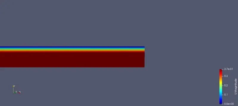
Velocity contour at the inlet and outlet of the pipe.
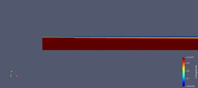
As seen from the above image, a velocity boundary layer is formed at the inlet as result of no-slip boundary condition in the internal surface of the pipe.
Plots showing velocity profile as function of pipe length in the hydrodynamically developing region.
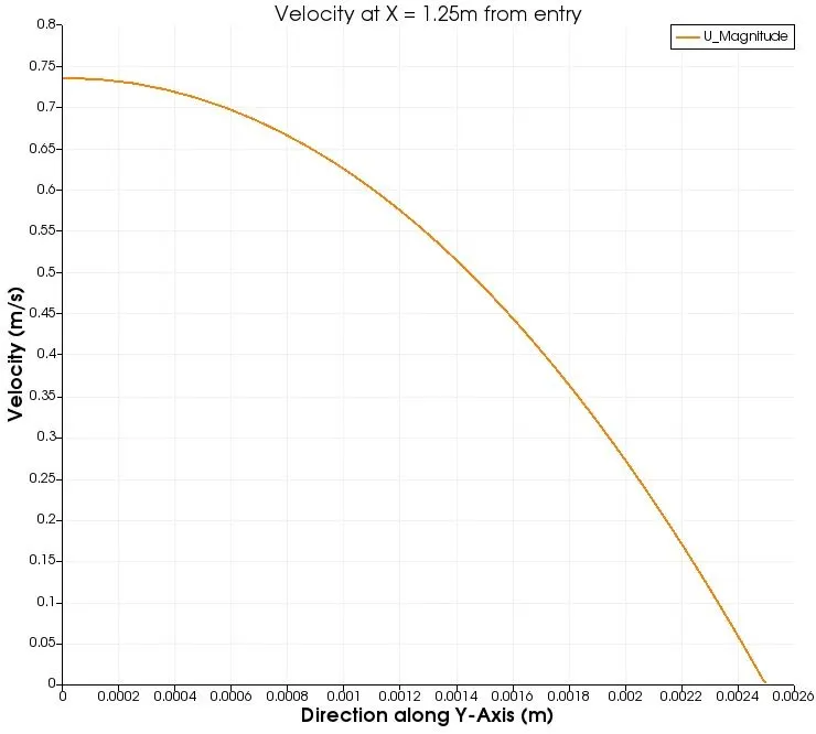
Plot showing velocity profile of fully developed flow
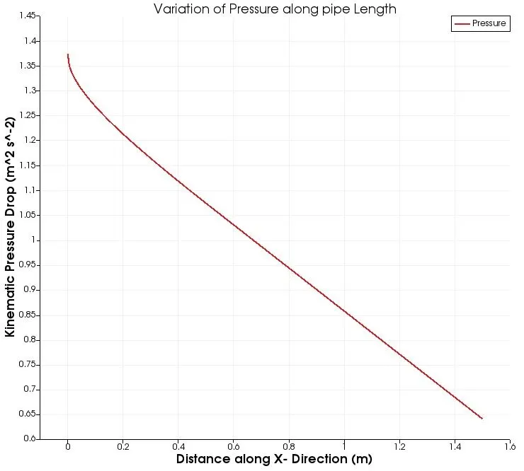
Plot showing Kinematic Pressure Drop along the length of the pipe
The validation of simulated results with analytical results are carried out using matlab by reading fully developed velocity data imported from Paraview in OpenFOAM. The code is given below
clear all
close all
clc

%Analytical velocity of fully developed flow

mu = 0.8891e-3;
U_avg = 0.3745;
r_max = 0.0025;
r = linspace(0,r_max,1001);

for i = 1:length(r)
    V_analytical(i) = 2*U_avg*(1-((r(i)^2)/(r_max^2)));
end

%Parsing Simulated data of fully developed velocity profile from Paraview

f1 = fopen('Vel_data.txt','r');
fgetl(f1);
A = fscanf(f1, '%f');
V = A(2:2:end);
V_simulated = V';
R = A(1:2:end);
r_1 = R';

%plot to validate simulated to anaytical velocity data

figure(1)
plot(V_analytical,r,'k')
hold on
plot(V_simulated, r_1,'r')
hold on
plot(V_analytical,-r,'k')
hold on
plot(V_simulated, -r_1,'r')
hold off
grid
title('Velocity profile of fully developed flow');
legend('Analytical','Simulated')
xlabel('Velocity (m/s)')
ylabel('Diameter (m)')

%Shear stress

for j = 2:length(r)
    Tau_analytical(j) = mu*((V_analytical(j-1)-V_analytical(j))/(r(j)-r(j-1)));
    Tau_simulated(j) = mu*((V_simulated(j-1)-V_simulated(j))/(r(j)-r(j-1)));
end

figure(2)
plot(Tau_analytical,r,'r')
hold on
plot(Tau_simulated,r,'k')
hold on
plot(Tau_analytical,-r,'r')
hold on
plot(Tau_simulated,-r,'k')
hold off
grid
title('Shear stress of fully developed flow');
legend('Analytical','Simulated')
xlabel('Shear Stress (Pa)')
ylabel('Diameter (m)')
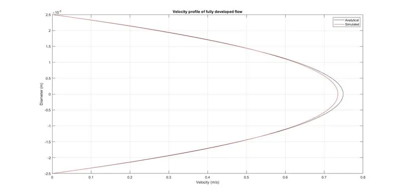
Plot showing validated results of Velocity
Plot showing validated results of Shear Stress
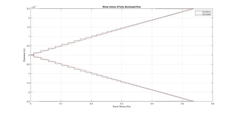
It can observed from the above plots that velocity of the flow is maximum at the centre of the pipe and zero at the wall surfaces due to no-slip boundary condition.The velocity profile is developed in such a way to satisfy the conservation of mass criteria. Since shear stress is inversely proportional to velocity, it can be observed that its magnitude is maximum at the inner surface of the pipe and minimum in the layer where velocity of the flow is at its maximum.