Challenge

Simulation of Flow through a pipe in OpenFOAM

UUjwal Sharma1 Nov 2021

Simulation an axi-symmetric flow by applying the wedge boundary condition. The flow is laminar and flows through a constant cross-section pipe at an inlet Reynold's number of 2100.Using a transient state simulation and validating that with Hagen- Poiseuille's equations for the fully developed flow.

Objective -

Write code in Matlab to automate the generation of blockMeshDict file.
Take neccessary details into consideration
Validate Hydro-dynamic length with the numerical result
Validate the fully developed flow velocity profile with its analytical profile
Validate maximum velocity and pressured drop for fully developed flow
Post-process Shear stress and validate wall shear stress for fully developed flow

Theory -

Wedge Boundary Condition

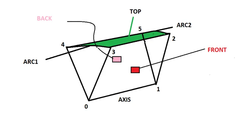
The wedge boundary condition (BC) is used in computational fluid dynamics to define an axisymmetric situation, for eg. cylinder. The model and flow must be axisymmetric along a central line such that all physical variables of the flow have the same value and distribution at a given radius for all angles.

This boundary condition is specified by two planes that must be selected on separate sides of the domain (referred to as front and back) on surfaces running along the axis.

Note -It works for 2D simulations only.

Poiseullie flow

Poiseullie flow is a pressure induced axisymmetric flow in a long plate of lenght(L). If the Poiseullie flow occurs in a circular pipe of lenght (L) and radius (R) then its called Hagen-Posieullie's flow.

Hagen-Posieullie's flow is analyzed using circular coordinates (r,`theta,0`) with origin on the centre line of the pipe entrance and z-direction aligned to centre of line.

Since we know that there is no exact solutiion for Navier Stokes equation. In order, to find the exact solution we take consideraton of the following assumptions

the flow is laminar,
Re=2100 and
`v_z!=0, v_r=0 & v_theta=0` we can also say that they negligible-Parallel Flow `

Consider fully developed laminar flow through a straight tube of circular cross-section as in figure below. Rotational symmetry is considered to make the flow two-dimensional axisymmetric.
Let us take z-axis as the axis of the tube along which all the fluid particles travel, i.e.

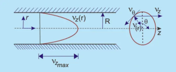
Hagen-Posieullie flow through a pipe

Now, from the continuity equation we obatin

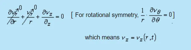
Invoking [`v_r=0,v_theta=0, (delv_z)/(delz)=0,&del/(deltheta)(anyquantity)=0`] in the

Navier Stokes equation we obtain,

`(delv_z)/(delt)=-1/rho+v((del^2v_z)/(delr^2)+1/r*(delv_z)/(delr))` in z-direction

For steady flow, governing equation becomes

`(del^2v_z)/(delr^2)+1/r*(delv)/(delr)=1/mu*(delrho)/(delz)`

Above obtained equation can we simplified as follows,

`r*(del^2v_z)/(delr^2)+(delv_z)/(delr)=1/mu*(delrho)/(delz)*r`

or `del/(delr)(r*(delv_z)/(delr))=1/mu*(delrho)/(delz)*r`

or `r*(delv_z)/(delr)=1/(2mu)(delrho)/(delz)*r^2+A`

or `(delv_z)/(delr)=1/(2mu)(delrho)/(delz)*r^2+A /r`

or `v_z=1/(4mu)*(delrho)/(delz)*r^2+A In(r+B)`

At r=0, `v_z` is finite which means 'A' should be be zero and at r=R, `v_z=0`

`B=1/(4mu)*(delrho)/(delr)*R^2`

i.e `v_z= R^2/(4mu)*(-(delrho)/(delz))(1-(r^2)/(R^2))`

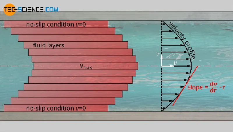
This shows that the axial velocity profile in a fully developed laminar pipe flow is having parabolic variation along r.

Therefore,

`(v_z)_(av)=R^2/(8mu)(-(delrho)/(delz))` Average Velocity

`(v_z)_max=2(v_z)_(av)` Maximium Velocity

`Q=(piD^4)/(128mu)*(delrho)/(delz)` Discharge rate

Codes -

clear all
close all
clc

%Given Data for Analysis
Re=2100; %Reynolds Number
mu=input("Enter Dynamic Viscosity of watern")
rho=input("Enter Density of watern")
d=input("Enter Diameter of pipen")
theta=input("Enter Wedge Angle for pipen")  %Wgde Andle should be <5 Degrees
  

%Entry Lenght of pipe
Le=d*(0.05*Re)
%Actual lenght of pipe
L=0.5+Le
R=d/2   %Radius of pipe
v_avg=(Re*mu)/(rho*d) %average velocity
v_max=2*v_avg  % maximium velocity
T_wall=4*((mu*v_avg)/R)
dp=(32*mu*v_avg)/((d)^2)
nu=mu/rho %Nuseltte Number
r=linspace(0,R,300);
v=v_max*(1-(r.^2./R^2));

plot(r,v,'linewidth',2)
xlabel('radius')
ylabel('velocity')
title('velocity profile at fully developed region')


%-------------------------------------------------------------------------------------------------------------------------------
%%writting the header part for BlockMeshDict File in Matlab
h1='/*--------------------------------*- C++ -*----------------------------------*';
h2='  =========                 |';
h3='        /  F ield         | OpenFOAM: The Open Source CFD Toolbox';
h4='       /   O peration     | Website:  https://openfoam.org';
h5='      /    A nd           | Version:  8';
h6='     /     M anipulation  |';
h7='*---------------------------------------------------------------------------*/';
h8='FoamFile';
h9='{';
h10='    version     2.0;';
h11='    format      ascii;';
h12='    class       dictionary;';
h13='    object      blockMeshDict;';
h14='}';
h15='// * * * * * * * * * * * * * * * * * * * * * * * * * * * * * * * * * * * * * //';
h16='// ************************************************************************* //';

conv='convertToMeters 1;';
v0=[0 0 0];
v1=[L 0 0];
v2=[L R*cosd(theta/2) R*sind(theta/2)];
v3=[0 R*cosd(theta/2) R*sind(theta/2)];
v4=[0 R*cosd(theta/2) -R*sind(theta/2)];
v5=[L R*cosd(theta/2) -R*sind(theta/2)];

block='hex (0 1 5 4 0 1 2 3) (500 20 1) simpleGrading (1 0.01 1)';
inlet='(0 1 2 0)';
outlet='(1 5 2 1)';
top='3 2 5 4';
front='0 1 2 3';
back='0 4 5 1';
axis='0 1 1 0';
s1=blanks(4);
s2=blanks(7);
s3=blanks(11);
s4=blanks(3);


%Generating blockMeshDict File
f1=fopen('blockMeshDict.txt','w');
fprintf(f1,'%sn',h1);
fprintf(f1,'%sn',h2);
fprintf(f1,'%sn',h3);
fprintf(f1,'%sn',h4);
fprintf(f1,'%sn',h5);
fprintf(f1,'%sn',h6);
fprintf(f1,'%sn',h7);
fprintf(f1,'%sn',h8);
fprintf(f1,'%sn',h9);
fprintf(f1,'%sn',h10); 
fprintf(f1,'%sn',h11); 
fprintf(f1,'%sn',h12);
fprintf(f1,'%sn',h13); 
fprintf(f1,'%sn',h14); 
fprintf(f1,'%sn',h15);
fprintf(f1,'n');

fprintf(f1,'%sn',conv);
fprintf(f1,'n');

fprintf(f1,'%sn','vertices');
fprintf(f1,'%sn','(');
fprintf(f1,'%s(%d %d %d)n',s1,v0(1),v0(2),v0(3));
fprintf(f1,'%s(%d %d %d)n',s1,v1(1),v1(2),v1(3));
fprintf(f1,'%s(%d %d %d)n',s1,v2(1),v2(2),v2(3));
fprintf(f1,'%s(%d %d %d)n',s1,v3(1),v3(2),v3(3));
fprintf(f1,'%s(%d %d %d)n',s1,v4(1),v4(2),v4(3));
fprintf(f1,'%s(%d %d %d)n',s1,v5(1),v5(2),v5(3));
fprintf(f1,'%sn',');');
fprintf(f1,'n');

fprintf(f1,'%sn','blocks');
fprintf(f1,'%sn','(');
fprintf(f1,'%s%sn',s4,block);
fprintf(f1,'n');
fprintf(f1,'%sn',');');
fprintf(f1,'n');

fprintf(f1,'%sn','edges');
fprintf(f1,'%sn','(');
fprintf(f1,'%s %s %d %d(%d %d %d)n',s4,'arc',3,4,0,R,0);
fprintf(f1,'%s %s %d %d(%d %d %d)n',s4,'arc',2,5,L,R,0);
fprintf(f1,'%sn',');');
fprintf(f1,'n');

fprintf(f1,'%sn','boundary');
fprintf(f1,'%sn','(');

fprintf(f1,'%s %sn',s4,'inlet');
fprintf(f1,'%s %sn',s4,'{');
fprintf(f1,'%s %sn',s2,'type patch;');
fprintf(f1,'%s %sn',s2,'faces');
fprintf(f1,'%s %sn',s2,'(');
fprintf(f1,'%s (%d %d %d %d)n',s3,0,3,4,0);
fprintf(f1,'%s %sn',s2,');');
fprintf(f1,'%s %sn',s4,'}');

fprintf(f1,'%s %sn',s4,'outlet');
fprintf(f1,'%s %sn',s4,'{');
fprintf(f1,'%s %sn',s2,'type patch;');
fprintf(f1,'%s %sn',s2,'faces');
fprintf(f1,'%s %sn',s2,'(');
fprintf(f1,'%s (%d %d %d %d)n',s3,1,5,2,1);
fprintf(f1,'%s %sn',s2,');');
fprintf(f1,'%s %sn',s4,'}');

fprintf(f1,'%s %sn',s4,'top');
fprintf(f1,'%s %sn',s4,'{');
fprintf(f1,'%s %sn',s2,'type wall;');
fprintf(f1,'%s %sn',s2,'faces');
fprintf(f1,'%s %sn',s2,'(');
fprintf(f1,'%s (%d %d %d %d)n',s3,3,2,5,4);
fprintf(f1,'%s %sn',s2,');');
fprintf(f1,'%s %sn',s4,'}');

fprintf(f1,'%s %sn',s4,'front');
fprintf(f1,'%s %sn',s4,'{');
fprintf(f1,'%s %sn',s2,'type wedge;');
fprintf(f1,'%s %sn',s2,'faces');
fprintf(f1,'%s %sn',s2,'(');
fprintf(f1,'%s (%d %d %d %d)n',s3,0,1,2,3);
fprintf(f1,'%s %sn',s2,');');
fprintf(f1,'%s %sn',s4,'}');

fprintf(f1,'%s %sn',s4,'back');
fprintf(f1,'%s %sn',s4,'{');
fprintf(f1,'%s %sn',s2,'type wedge;');
fprintf(f1,'%s %sn',s2,'faces');
fprintf(f1,'%s %sn',s2,'(');
fprintf(f1,'%s (%d %d %d %d)n',s3,0,4,5,1);
fprintf(f1,'%s %sn',s2,');');
fprintf(f1,'%s %sn',s4,'}');

fprintf(f1,'%s %sn',s4,'axis');
fprintf(f1,'%s %sn',s4,'{');
fprintf(f1,'%s %sn',s2,'type empty;');
fprintf(f1,'%s %sn',s2,'faces');
fprintf(f1,'%s %sn',s2,'(');
fprintf(f1,'%s (%d %d %d %d)n',s3,0,1,1,0);
fprintf(f1,'%s %sn',s2,');');
fprintf(f1,'%s %sn',s4,'}');
fprintf(f1,'%sn',s2,');');
fprintf(f1,'n');
fprintf(f1,'%sn','mergePatchPairs');
fprintf(f1,'%sn','(');
fprintf(f1,'%sn',');');

fprintf(f1,'%sn',h16);
fclose(f1);
%---------------------------------------------------------------------------------------------------------------------------

blockMeshDict File

/*--------------------------------*- C++ -*----------------------------------*
  =========                 |
        /  F ield         | OpenFOAM: The Open Source CFD Toolbox
       /   O peration     | Website:  https://openfoam.org
      /    A nd           | Version:  8
     /     M anipulation  |
*---------------------------------------------------------------------------*/
FoamFile
{
    version     2.0;
    format      ascii;
    class       dictionary;
    object      blockMeshDict;
}
// * * * * * * * * * * * * * * * * * * * * * * * * * * * * * * * * * * * * * //

convertToMeters 1;

vertices
(
    (0 0 0)
    (2.600000e+00 0 0)
    (2.600000e+00 9.998477e-03 1.745241e-04)
    (0 9.998477e-03 1.745241e-04)
    (0 9.998477e-03 -1.745241e-04)
    (2.600000e+00 9.998477e-03 -1.745241e-04)
);

blocks
(
   hex (0 1 5 4 0 1 2 3) (500 20 1) simpleGrading (10 0.01 1)

);

edges
(
    arc 3 4(0 1.000000e-02 0)
    arc 2 5(2.600000e+00 1.000000e-02 0)
);

boundary
(
    inlet
    {
        type patch;
        faces
        (
            (0 3 4 0)
        );
    }
    outlet
    {
        type patch;
        faces
        (
            (1 5 2 1)
        );
    }
    top
    {
        type wall;
        faces
        (
            (3 2 5 4)
        );
    }
    front
    {
        type wedge;
        faces
        (
            (0 1 2 3)
        );
    }
    back
    {
        type wedge;
        faces
        (
            (0 4 5 1)
        );
    }
    axis
    {
        type empty;
        faces
        (
            (0 1 1 0)
        );
    }
       
);

mergePatchPairs
(
);
// ************************************************************************* //

P(Pressure File) -

/*--------------------------------*- C++ -*----------------------------------*
  =========                 |
        /  F ield         | OpenFOAM: The Open Source CFD Toolbox
       /   O peration     | Website:  https://openfoam.org
      /    A nd           | Version:  8
     /     M anipulation  |
*---------------------------------------------------------------------------*/
FoamFile
{
    version     2.0;
    format      ascii;
    class       volScalarField;
    object      p;
}
// * * * * * * * * * * * * * * * * * * * * * * * * * * * * * * * * * * * * * //

dimensions      [0 2 -2 0 0 0 0];

internalField   uniform 0;

boundaryField
{
    inlet
    {
        type            zeroGradient;
    }

    outlet
    {
        type            fixedValue;
        value           uniform;
    }

    front
    {
        type            wedge;
    }
    
    back
    {
        type            wedge;
    }
    
    top
    {
        type            zeroGradient;
    }
    
    axis
    {
        type            empty;
    }
}
// ************************************************************************* //

U(Velocity File)-

/*--------------------------------*- C++ -*----------------------------------*
  =========                 |
        /  F ield         | OpenFOAM: The Open Source CFD Toolbox
       /   O peration     | Website:  https://openfoam.org
      /    A nd           | Version:  8
     /     M anipulation  |
*---------------------------------------------------------------------------*/
FoamFile
{
    version     2.0;
    format      ascii;
    class       volVectorField;
    object      U;
}
// * * * * * * * * * * * * * * * * * * * * * * * * * * * * * * * * * * * * * //

dimensions      [0 1 -1 0 0 0 0];

internalField   uniform (0.11 0 0);

boundaryField
{
    inlet
    {
        type            fixedValue;
        value           uniform (0.11 0 0);
    }
    
    outlet
    {
        type            zeroGradient;
    }
    
    front
    {
        type            wedge;
    }
    
    back
    {
        type            wedge;
    }

    top
    {
        type            noSlip;
    }

    axis
    {
        type            empty;
    }
    
}

// ************************************************************************* //

ControlDict File -

/*--------------------------------*- C++ -*----------------------------------*
  =========                 |
        /  F ield         | OpenFOAM: The Open Source CFD Toolbox
       /   O peration     | Website:  https://openfoam.org
      /    A nd           | Version:  8
     /     M anipulation  |
*---------------------------------------------------------------------------*/
FoamFile
{
    version     2.0;
    format      ascii;
    class       dictionary;
    location    "system";
    object      controlDict;
}
// * * * * * * * * * * * * * * * * * * * * * * * * * * * * * * * * * * * * * //

application     icoFoam;

startFrom       startTime;

startTime       0;

stopAt          endTime;

endTime         50;

deltaT          0.005;

writeControl    timeStep;

writeInterval   20;

purgeWrite      0;

writeFormat     ascii;

writePrecision  6;

writeCompression off;

timeFormat      general;

timePrecision   6;

runTimeModifiable true;


// ************************************************************************* //

TransportProperties-

/*--------------------------------*- C++ -*----------------------------------*
  =========                 |
        /  F ield         | OpenFOAM: The Open Source CFD Toolbox
       /   O peration     | Website:  https://openfoam.org
      /    A nd           | Version:  8
     /     M anipulation  |
*---------------------------------------------------------------------------*/
FoamFile
{
    version     2.0;
    format      ascii;
    class       dictionary;
    location    "constant";
    object      transportProperties;
}
// * * * * * * * * * * * * * * * * * * * * * * * * * * * * * * * * * * * * * //

nu              [0 2 -1 0 0 0 0] 8.97e-7;


// ************************************************************************* //

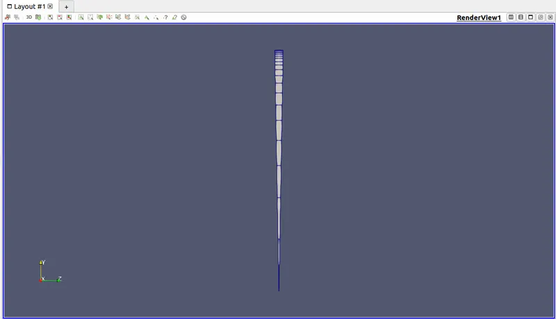
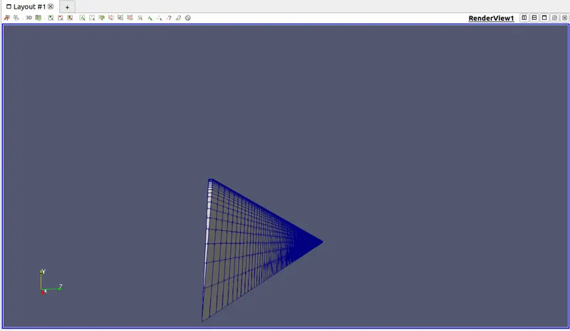
Geometry generated -

Before Refinement -

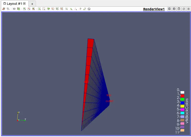
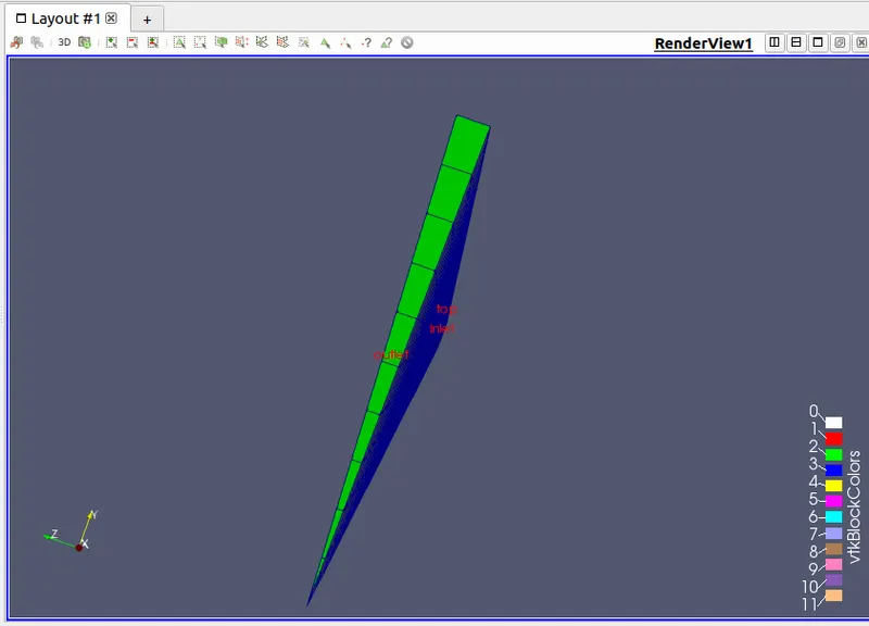
After Refinement -

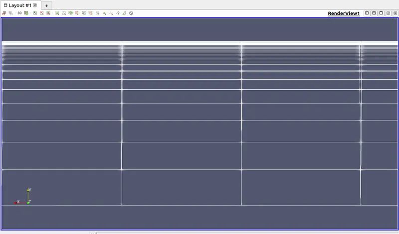
Mesh Generated -

Before Refinement -

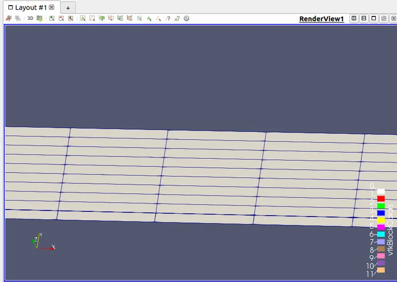
After Refinement -

Theoretical Calculation -

Enter Dynamic Viscosity of water
8.9e-4

mu =

   8.9000e-04

Enter Density of water
997

rho =

   997

Enter Diameter of pipe
0.02

d =

    0.0200

Enter Wedge Angle for pipe
3

theta =

     3


Le =

    2.1000


L =

    2.6000


R =

    0.0100


vz_avg =

    0.0937


vz_max =

    0.1875


T_wall =

    0.0334


dp =

    6.6737


nu =

   8.9268e-07

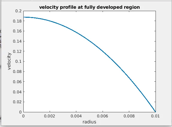
Theoretical full developed velocity profile -

Simulation solution full developed Velocity Profile-

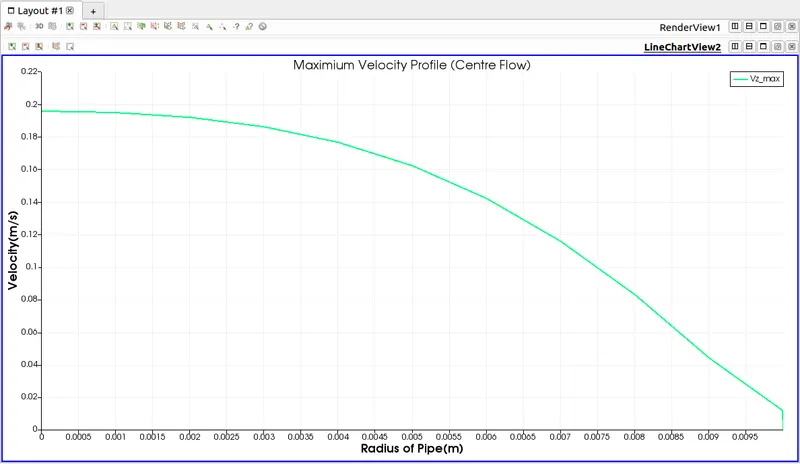
Velocity Profile obtained from the simulation -

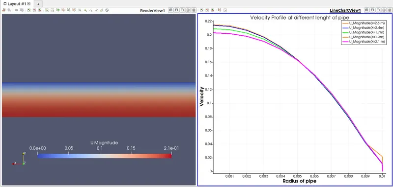
If one observes the plot velocity magnitude plot, its a comparsion at different lengths but after X=2.4 almost every other increment so the length overlaps the pervious plot. Hence we obtain an hydro-dynamic length (Le)=2.4.

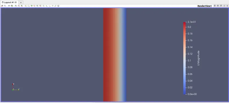
This picture determines U_mag obtained after 50 i.e endTime for the simulation solution.

Pressure Drop -

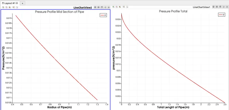
Note - In the Mid Section plot the X-axis is not Radius of pipe but its the Mid section length from inlet to mid Horizon.

T_wall or Shear Stress -

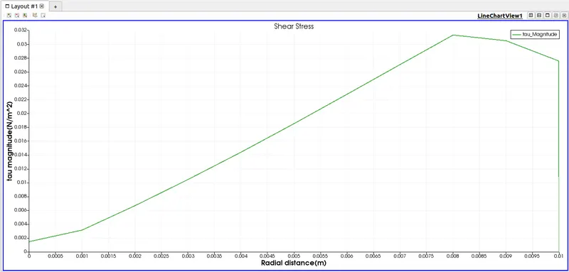
The Newton's constitutive law, for any general geometry states that the shear tensor (second_order tensor) is proportional to the flow velocity gradient. And the constants of proportionality is named dynamic viscosity(the velocity is a vector, so its gradient is second-order tensor).

`tau=-mu*(du)/(dy)`

negative sign denotes the direction of shear stress.

Note- As we move away from the centre axis ,Shear strerss increases. Thus, we can say that shear stress at pipe walls are high.

Vadidation -

Paramters	Numerical Soln	Theoretical Soln
V_max	0.195 m/s	0.1875 m/s
Velocity Profile	Parabolic	Parabolic
Le	2.4 m	2.1 m
T_wall	0.03199 N/m^2	0.0334 N/m^2

Conclusion -

The Shear Stress plot displays a sudden dip in the graph after a gradual rise, This is due to mesh of geometry.
In our case the Shear Stress dip until it touches the axis i.e 0.01m , this happens due to the refinement of the mesh geometry is High.
The Shear Stress plot displays a sudden dip in the graph after a gradual rise, This is due to mesh of geometry.
Shear Stress decrease as we approach the centre of the pipe whereas increases towards the walls(Noslip) of pipe.
Velocity is maximium at the centre of the pipe and decreases in the magnitude as we try to measure the velocity closes to that of walls , This due to the viscosity of the fluid medium inside the pipe.

Reference -

Matlab parsing file - https://skill-lync.com/premium/coursevideos/47435/en/1513
Velocity Profile Plotting - https://skill-lync.com/knowledgebase/how-to-create-plot-over-line-in-paraview
T_wall or Shear Stress Plotting - https://skill-lync.com/knowledgebase/how-to-create-shear-stress-plot-inside-paraview
Hagen-Posieullie Equation derivation and concepts - https://nptel.ac.in/content/storage2/courses/112104118/lecture-26/26-3_hag_poiseuille.htm -https://www.tec-science.com/mechanics/gases-and-liquids/hagen-poiseuille-equation-for-pipe-flows-with-friction/
Simplifying the Navier Stokes equation and understanding the Velocity distribution with solved examples - http://web.mit.edu/snively/www/2_006%20Coursenotes.pdf
Mesh Generation -https://cfd.direct/openfoam/user-guide/v6-blockmesh/

Simulation of Flow through a pipe in OpenFOAM

Ship work like this
in your own course.

Talk to a career counsellor

Ship work like thisin your own course.

Talk to a career counsellor

Ship work like this
in your own course.