Week 8 - Simulation of a backward facing step in OpenFOAM
AIM: The assignment aims to simulate a backward facing step using OPENFOAM. The simulation is an incompressible laminar viscous flow through a backward facing step geometry.
TOOLS USED: OPENFOAM
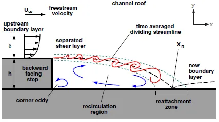
THEORY: The simulation of a backward facing step is a very crucial CFD simulation problem which gives us a good understanding of flow separation and re-attachment phenomenon. Consider the figure of the BFS
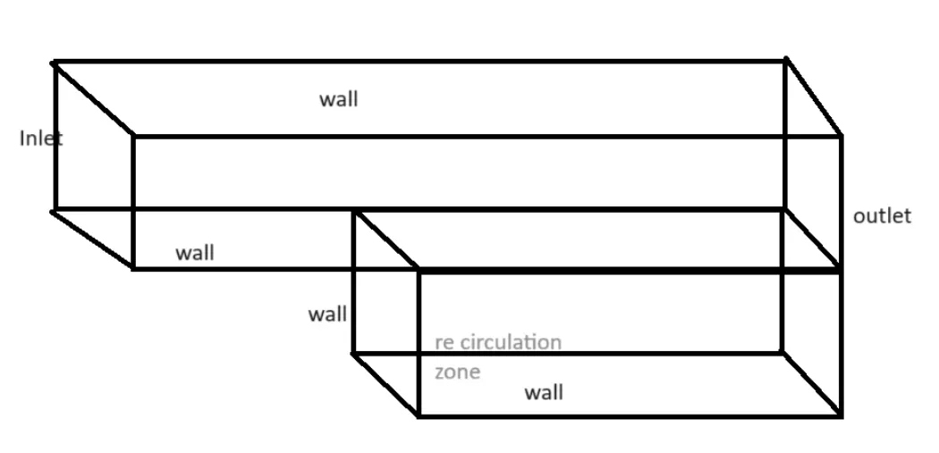
Here you can see the inlet where the flow comes. The flow separates at the step edge, creating a recirculation zone downstream. The flow eventually reattaches further downstream, forming a complex structure of separated and reattaching flow that is sensitive to initial and boundary conditions.
Depending on the Reynolds number, the flow can be laminar or turbulent and can exhibit complex turbulent structures like vortices or eddies.
STEPS :
1. The first step is to go inside the folder where there are different tutorials for OpenFoam.
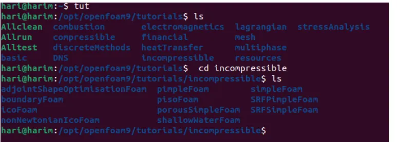
'tut' gives a list of all the Openfoam tutorials available. We then select then incompressible folder. To access the folder we type ' cd
2. We go inside the 'icoFoam' folder inside the 'incompressible' folder. we need to use the folder cavity. We cannot tamper the file inside openfoam tutorials , so we need to make a copy of the file , rename and run the simulations.

to copy the file, we use the command : cp -r
3. Now once we have the copy of the cavity, we can start working on the problem. when we go inside the cavity folder, we can see a few files.
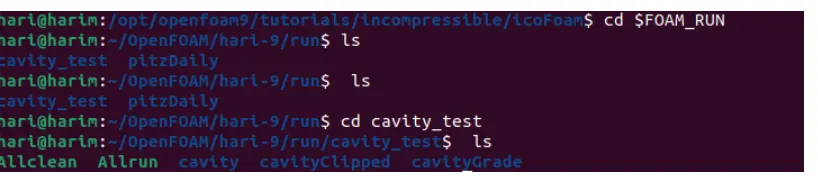
4. we go to the file cavity and go inside system and list all the files and we see this.
The blockMeshDict is the file that is used to work on the geometry and the mesh.

We open the BlockMeshDict file and tweak the model geometry.
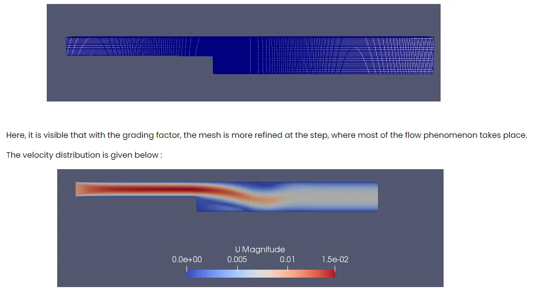
We run the simulations as two cases. One without the gradient factor and one with the gradient factor and see how the simulation is different: The coordinates of the geometry is given below:
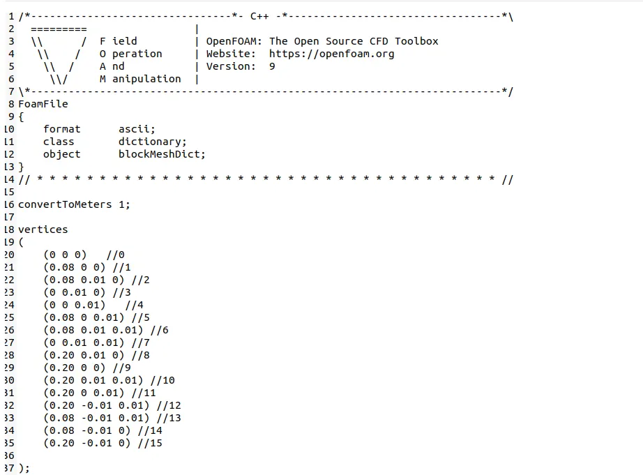
The figure is as shown below :
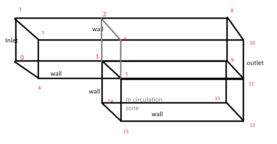
The same figure is used for both the cases. Now coming to the mesh,
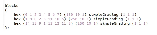
Here we use a hexahedral mesh. The notation hex ( n1 n1 n3 ......) gives the indices in an anticlockwise manner in such a way the the normal points out of the domain. We have three three blocks, so we have three hex commands. The simple grading is not there, so you see (1 1 1 ).
We assign the boundaries as per the right hand thumb rule :
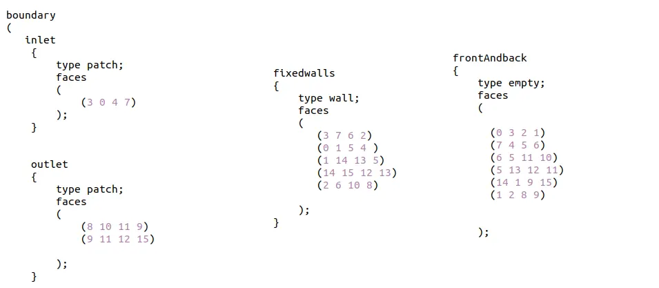
Pressure boundary conditions
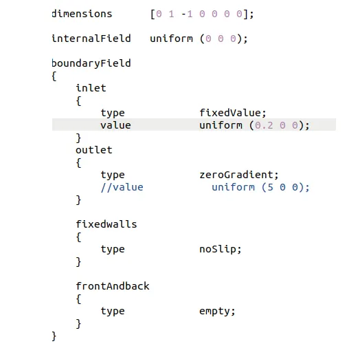
The velocity Boundary conditions:
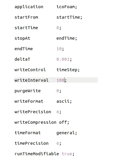
SOLVER
The solver used is the icoFoam. This is used to solve the incompressible Navier Stokes Equation using the PISO algorithm. The code is usually transient.
RESULTS AND DISCUSSION
1. Without grading factor
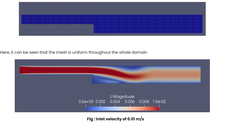
The above figure is the velocity distribution inside the BFS at the end of 10 seconds. You can observe that the flow has detached at the step and re-attaches further downstream.
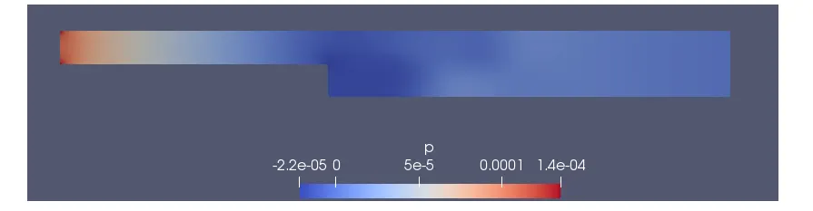
The pressure distribution is shown in the above figure.
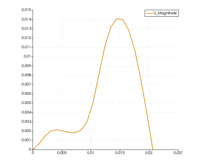
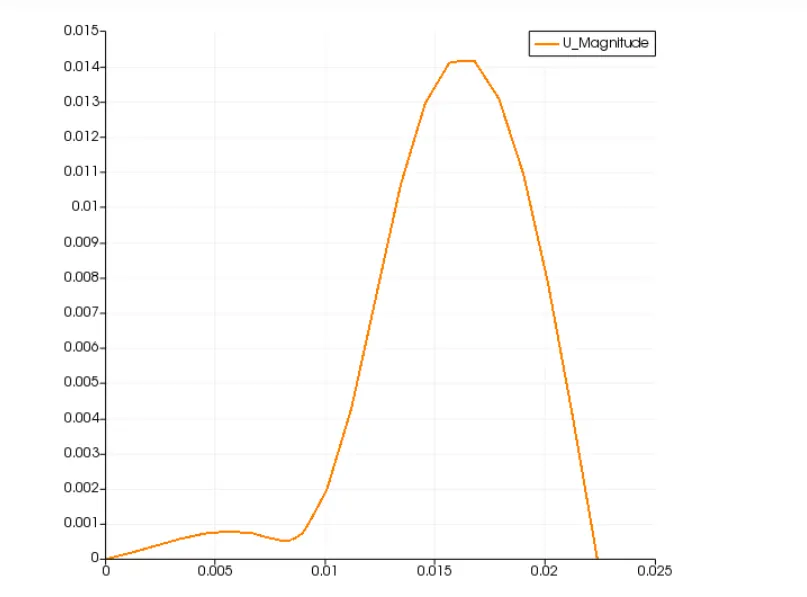
The plot above shows the maximum value of velocity at the proximity of the step.
2. With Grading factor
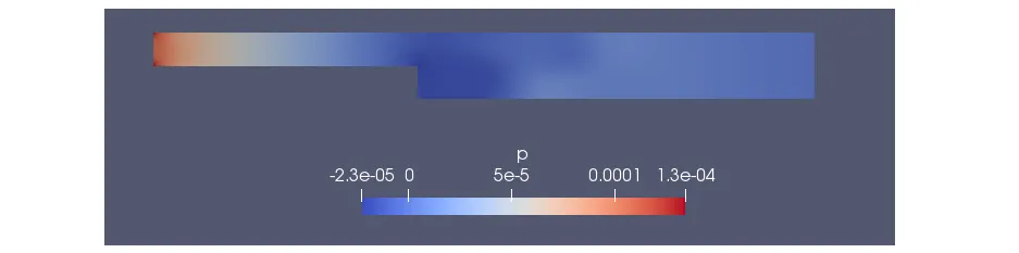
The pressure distribution is
The velocity magnitude of velocity in the proximity of the step is given below.