Week 8 - Simulation of a backward facing step in OpenFOAM

AIM

To simulate an incompressible-laminar-viscous flow through the backward facing step geometry. Perform a transient simulation and choose the inlet velocity such that the flow is laminar.

After that perform 2 case studies as described below and compare the results.

Case 1 - Simulate the flow without using any grading factor (i.e., GF = 1)

Case 2 - Simulate the flow with grading factor of 0.2. The cells should be finer near the walls (includig the step wall).

Mesh specification

1. Number of cells along the x direction (longer dimension) = 200
2. Number of cells along the longer y direction = 20;

Boundary condition specification

The domain specifications are provided in the following figure.

BODY OF CONTENT

• Lets start with the opening of the tutorial file in the terminal window

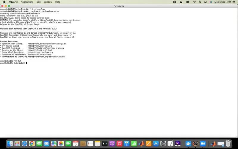
• Then we list the tutorials and then we select the directory incompressible from it.
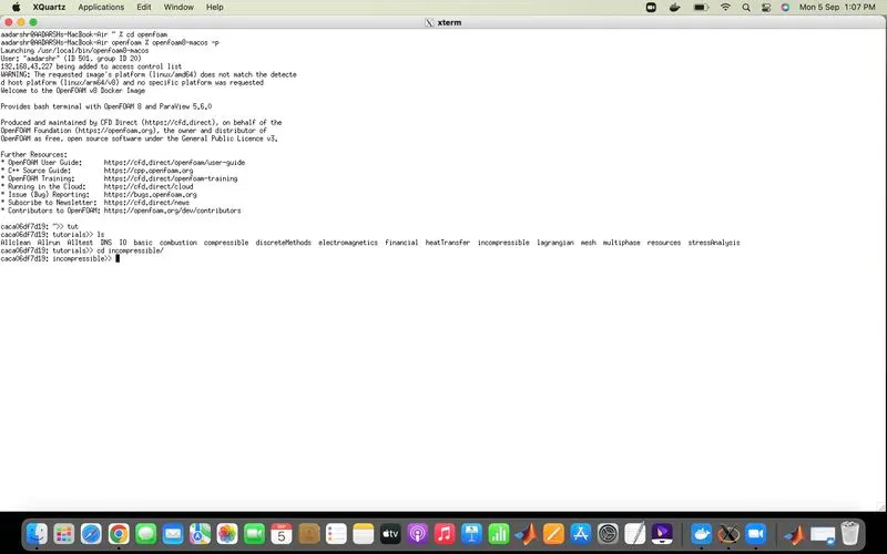
• The selection of the directory incompressible is carried out using the cd command which is called 'create directory'.

• Inside the incompressible directory we take the solver icofoam, which is the incompressible Navier Stokes equation.
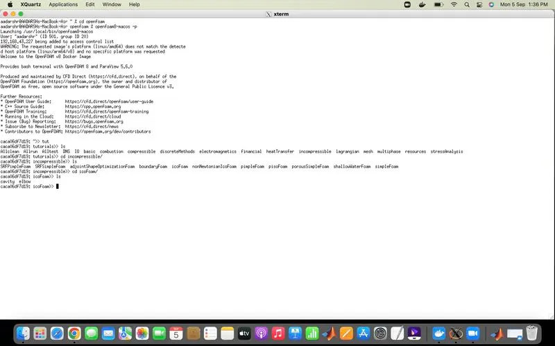
• Here we are solving only continuity and momentum equation using the icoFoam solver. Inside the solver icoFoam we have our required directories cavity and elbow, they both are part of the icoFoam solver and cavity section use to create required domain and black mesh so we choose cavity directory inside which we have another cavity folder, where we have to define our fluid domain and generate block mesh.

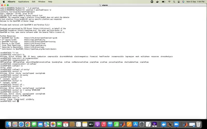
• Now we have to copy the main directory into the run folder using the command cp -r cavity/ $FOAM_RUN where 'cp' is the command to copy the folder cavity to the folder 'run'. We do that because inside the tutorial file we cannot run our program. Running it inside the tutorial results in the messing up of the inbuilt values of the specified solver.

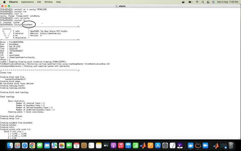
• Here we type a command called blockMesh to check for the various features and dimensions of the present in the equation, also the mesh information and boundary information are also provided.
• Then we type the icoFoam command and execute the program inside the terminal which is then copied into the paraview using 'paraFoam' command.

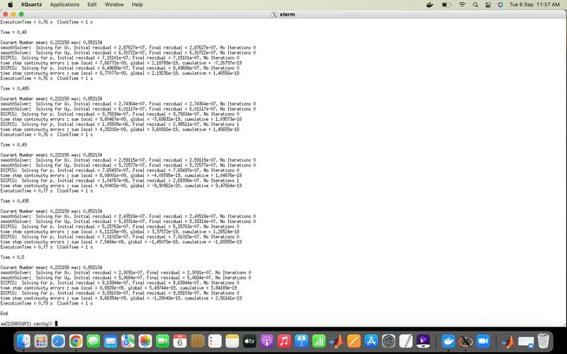
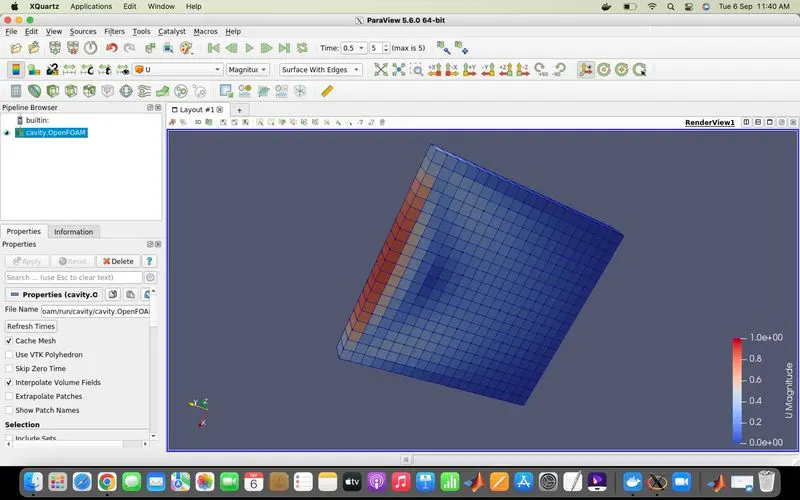
• The above image is the representation of incompressible laminar flow of a cavity surface using paraview.
• Now let us begin to create the backward facing step using the specified geometry for that we have to first edit the blockmesh dict file which is inside the system folder. At first we have to change the vertices, the boundary conditions, the input and output conditions by making changes in the blockmeshdict file as per the specified details.

At first we change the vertices of the backward facing step as given in the figure

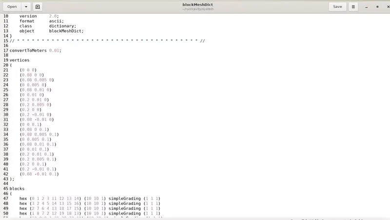
• In the above image we created the vertices of the backward facing step. It consists of 22 vertices, the first one of which is termed as point 0, which is the orign with values 0,0,0 at x,y and z axes.
• Then the next vertex is given as per the given figure of the step, where the total length of the step is 0.2m and the length of the right side of the step is 0.12m which makes the x axis from left 0.08m. Thus we take the x axis for the back side as 0.08, yaxis as 0 and z axis as 0.

Similarly the height of the side block is given as 0.01m , since we have 5 cells as shown we take the hight of cells 1, 2, 3 and 4 as 0.005 andc cell 5 as 0.01

Now let us index the cells as shown below

The above image is the back side of the Blocks, Since openFoam uses C++ programming, we start the index from '0'. Then we index the front side which is shown below

In the front side we give vertices at the z axis as 0.1

(0 0 0.1)
(0.08 0 0.1)
(0.08 0.005 0.1)
(0 0.005 0.1)
(0.08 0.01 0.1)
(0 0.01 0.1)
(0.2 0.01 0.1)
(0.2 0.005 0.1)
(0.2 0 0.1)
(0.2 -0.01 0.1)
(0.08 -0.01 0.1)

This results in making the front and back side of the step figure as shown which is the required one

Then we define the blocks, for that we need to specify the right order of vertex indices

For example:

to create the 1st Block for this case,

hex (0 1 2 3 11 12 13 14) (10 10 1) simpleGrading (1 1 1)

Similarly proceed by defining the vertices of the other blocks in the Geometry. At first we give 10 number of grid cells for x and y axis and then we give number of grid cells along x direction as 200 and along y direction as 20

blocks
(
hex (0 1 2 3 11 12 13 14) (80 5 1) simpleGrading (1 1 1)
hex (3 2 4 5 14 13 15 16) (80 5 1) simpleGrading (1 1 1)
hex (2 7 6 4 13 18 17 15) (120 5 1) simpleGrading (1 1 1)
hex (1 8 7 2 12 19 18 13) (120 5 1) simpleGrading (1 1 1)
hex (10 9 8 1 21 20 19 12) (120 10 1) simpleGrading (1 1 1)
);

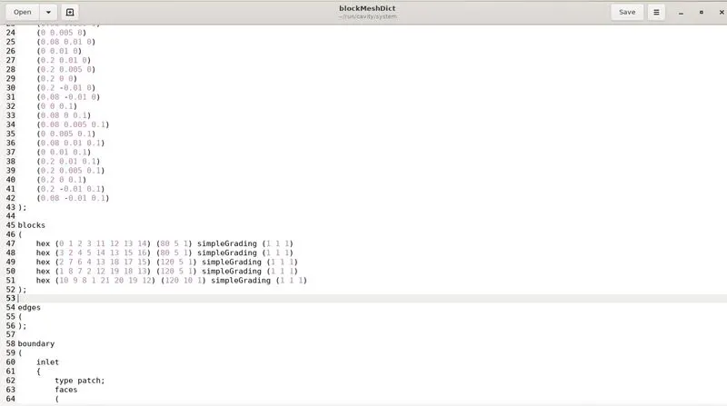
• In the above command hex stands for hexahedral and inside it we give our vertices and then we give the number of grid cells, here we give 80 grid cells in x axis and 5 grid cells on y axis so that the number of grid cell in the x direction becomes 200 and y direction becomes 20. This is done for all the 5 sections given in the step.
• Now we give the boundary conditions for that first we give inlet boundary condition as shown

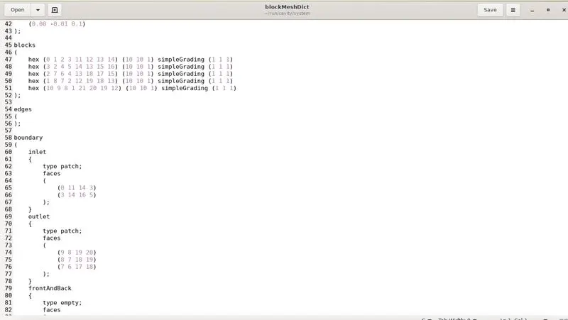
Here the inlet is given the type patch and the faces are given as the right hand rule i.e If we are looking at these faces from the outside, the definition of inlet boundary will be in counter-clockwise direction,

(0 11 14 3)

(3 14 16 5)

• Similarly, we have 3 faces contributing to the outlet boundary condition. Since we are viewing the faces from outside, hence the definition of the outlet boundary will be in counter-clockwise direction,

(9 8 19 20)

(8 7 18 19)

(7 6 17 18)

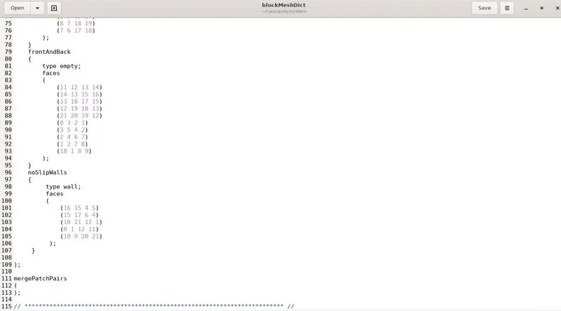
Then we define the front and back side of the step in the similar manner and also we have the no slip walls which again we define in the similar manner.

Front & Back

• In the above figure the front and back boundary conditions are shown as the vertices of the corresponding parts are defined as per the requirement.

No Slip walls

• Here we define the walls where no slip condition is applicable

• Now we change the dt in the controlDict folder where we have the start time, end time, the name of the solver used and time step are given. But we change the time step as per our requirement and to remove the error caused due to increase in Courant number.

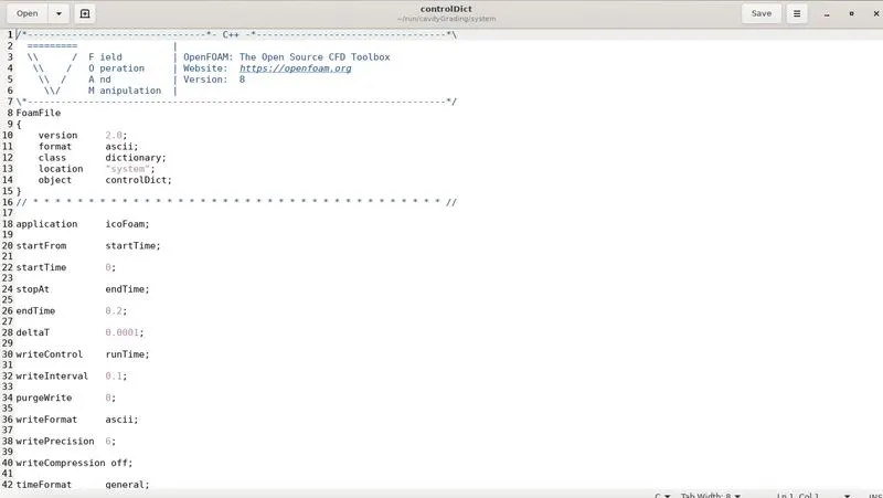
• In the above image we changed the time step deltaT so that it helps to remove the error caused due to increase in Courant number.

• Then, we have to define initial value for pressure and velocity. In order to do that, we have to go back in cavity directory using ‘cd ..’ command and select folder named ‘0’, which stand for initial values. In this case initial value for pressure and velocity.

• In this case,we have to set initial boundary condition for pressure and velocity at each faces also update the name of the boundary same as we changed inlet outlet name in ‘blockMeshDict’ script file as per shown in below codes.

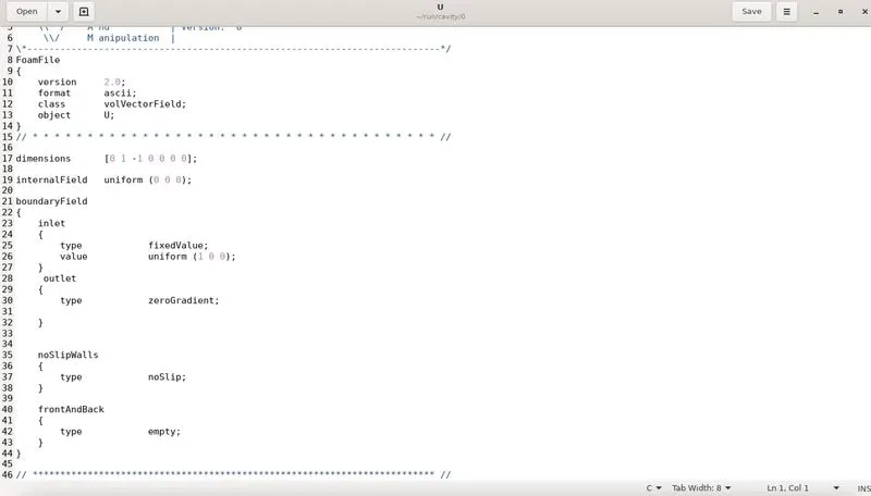
• Here we give the type fixedValue in the inlet because the velocity inside the cells at the inlet are uniform and at the outlet it is of type zeroGradient .
• Now we set the initial pressure at each faces, using the gedit command.

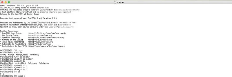
• Using the command results in the opening of the pressure window which we set according to our requirement.

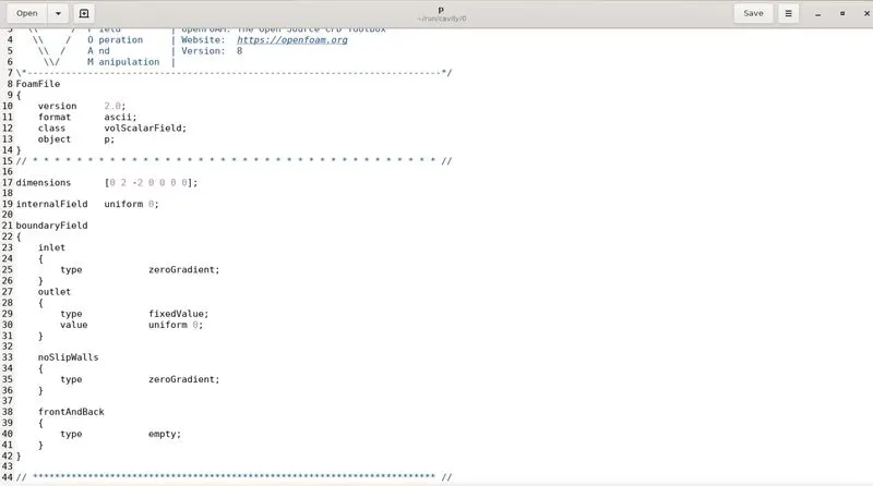
• Here we give the type zerogradient because the pressure inside the cells are uniform and there is no change in pressure thus pressure gradient is given as zeroGradient.
• Now we create the plot that is required by running the program, inorder to do that we need to give a command called icoFoam which runs the program, because it is the solver used in the current program.

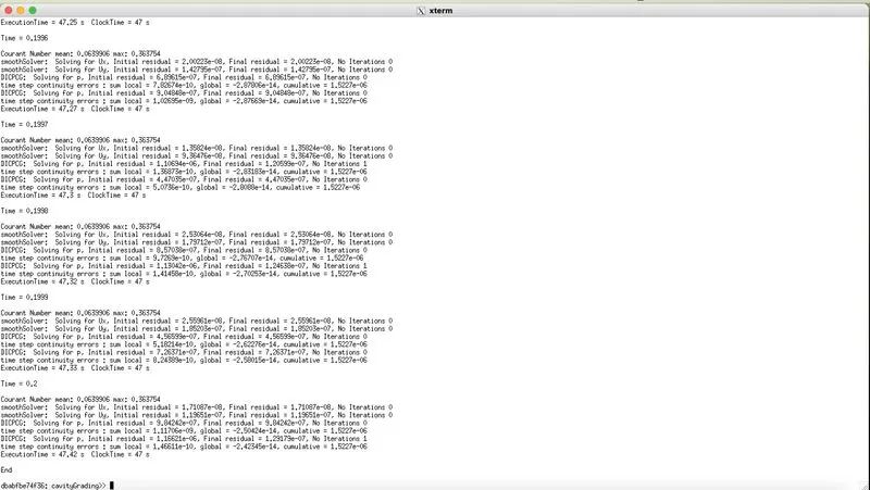
• After executing the command the backward step equation runs and shows the information that are calculated along with it which is shown in the above image. Then we write a command called paraFoam which is used to display the backward facing step in the paraview file.

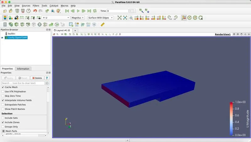
• The above image is the pictorial representation of initial velocity flowing through the backward facing step
• Then we execute the run command by clicking on the play button which results in the variation of velocity at different time steps and at end time 0.2.
• The below shown image is the simulation of the flow without using any grading factor (i.e., GF = 1)

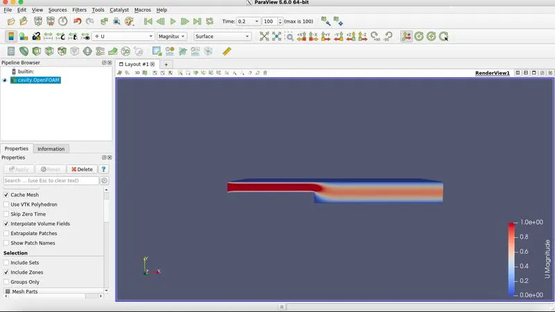
• At the right bottom side we have the variation of the velocity with respect to the colour variation is explained which varies from 0 to 1.
• Then we find the pressure variation with respect to different time steps till time 0.2

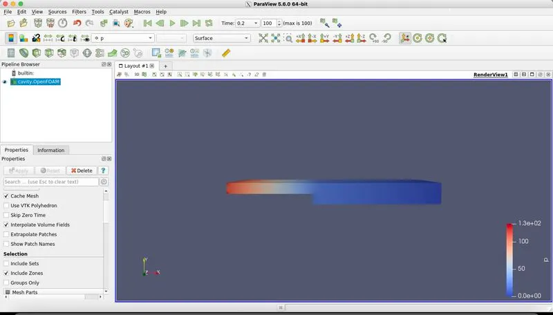
• Then we simulate the flow with grading factor of 0.2. The cells should be finer near the walls (includig the step wall).
• This change in grading factor is done inside the blockmeshDict file as shown below

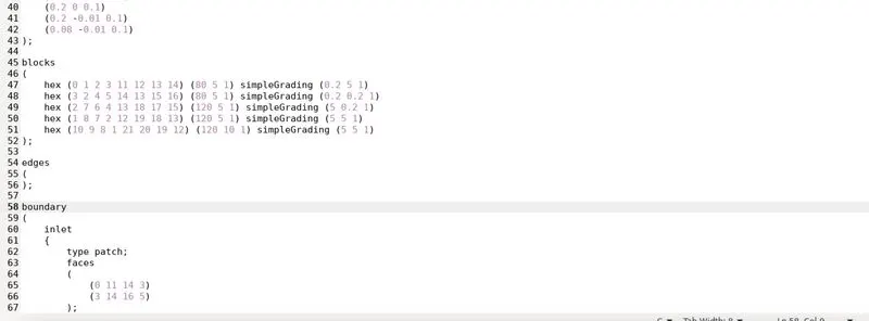
• In the above image we changed the simpleGrading (1 1 1) into (0.2 5 1) so that the cells are finer near the walls, includig the step wall. This grading results in converting the size of the cells at the end 20 times smaller than the size of the starting cell which is shown below

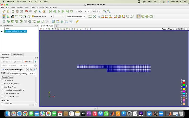
• In the above image we can see that the size of the cells near the walls, including the step wall are smaller than the size of the cells at the beginning which is to be shown as per the requirement
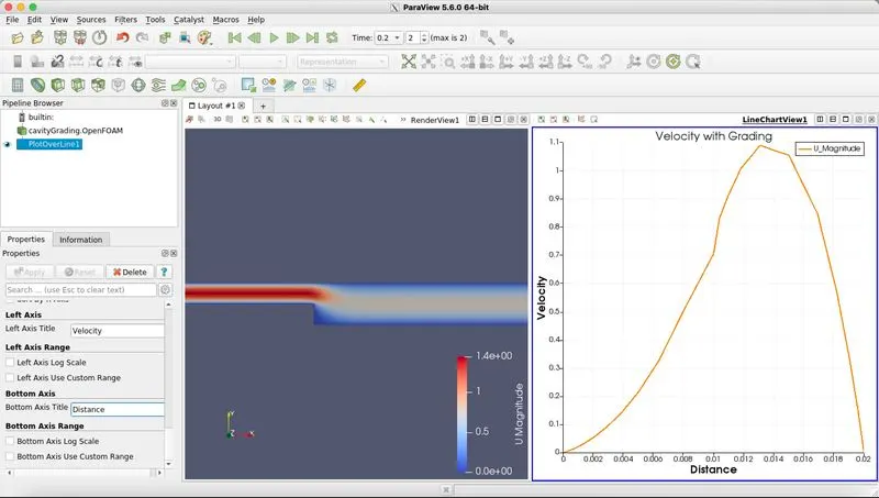
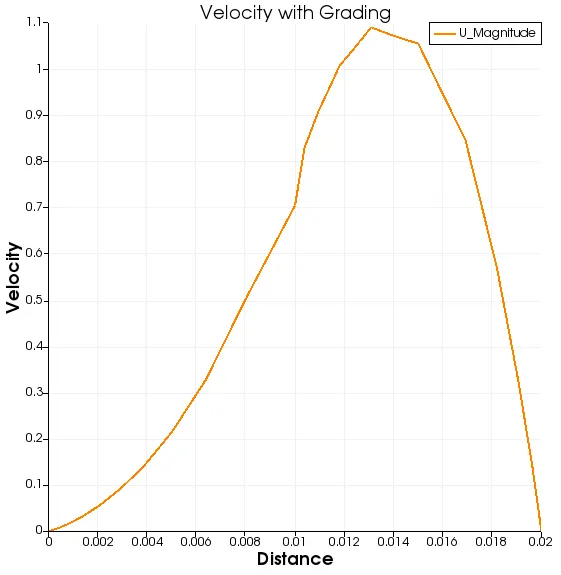
• Now we measure the velocity profile at 0.085 m from the inlet of the geometry for both case studies and compare by using the plot over line tool for this.
• For that purpose we click on the plot over line tool present on the top of the image

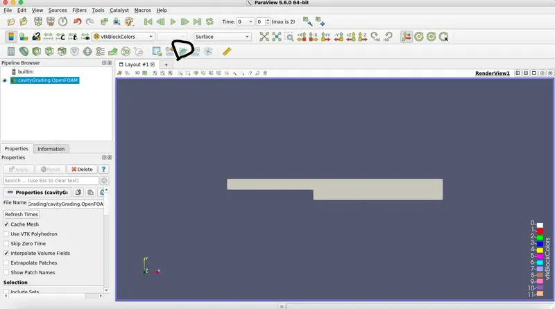
• By clicking on the tool an axis along with it's dimensions pops out and we change the direction of the axis parallel to y direction and then change the dimension of x axis and y axis as 0.085 and then we click apply button which results in popping of a graph which measures velocity against distance.

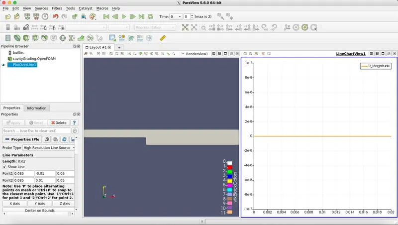
• Then we run the program from time 0 to 0.2 which shows the required plot of velocity profile.

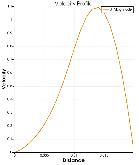
• The above shown is the velocity profile of the sample without grading i.e at grading factor =1

• Then we plot the velocity profile of the sample with grading factor = 0.2

RESULT

By comparing the two plot we can see that velocity profile without the grading factor is smoother than the profile with grading factor. But in actual case grading factor helps us to stretch the mesh along one direction and is useful for computational efficiency.In CFD fluid always shows large changes near walls and obstacles along its way and to capture those changes effectively we should always use grading or finer mesh near a wall.

Grading Factor = size of end cell/size of starting cell

If Grading factor = 0.1 it means thhat the end cell is 10 times smaller than the starting cell.