Project 1 - Parsing NASA thermodynamic data
REPORT ON PROJECT PARSING NASA THERMODYNAMIC DATA
AIM
To write a program that parse NASA Thermodynamic data and to calculate the thermodynamic properties such as Specific heat 'Cp', Enthalpy 'h' and Entropy 's' and also to plot the same against local temperature 't'
OBJECTIVE
- Write a function that extracts the 14 co-efficients and calculates the enthalpy, entropy and specific heats for all the species in the data file. The formulae are shown below.
Cp/R = a1+a2*(t)+a3*(t.^2)+a4*(t.^3)+a5*(t.^4)
H/Rt = (a1+a2*(t./2)+a3*((t.^2)./3)+a4*((t.^3)./4)+a5*((t.^4)./5)+a6./t)
S/R = (a1*log(t)+a2.*t+a3*((t.^2)./2)+a4*((t.^3)./3)+a5*((t.^4)./4)+a7)
Here R is the universal gas constant
- Calculate the molecular weight of each species and display it in the command window.
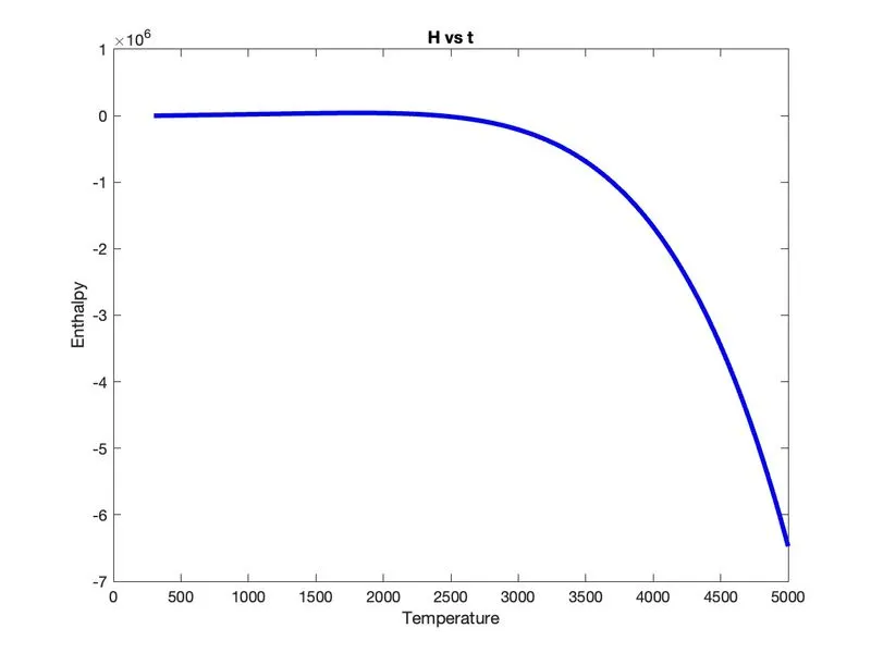
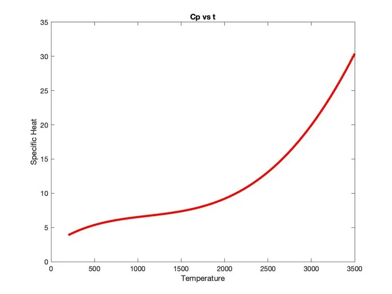
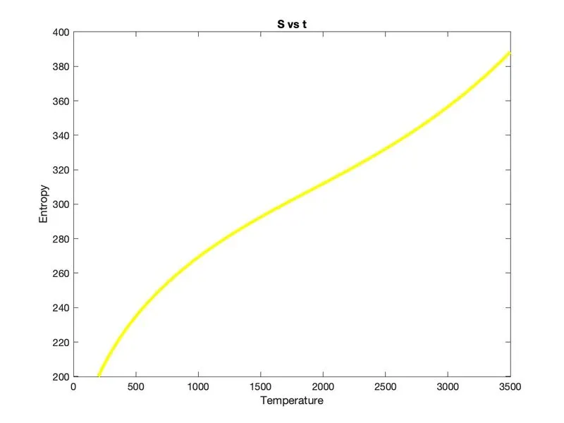
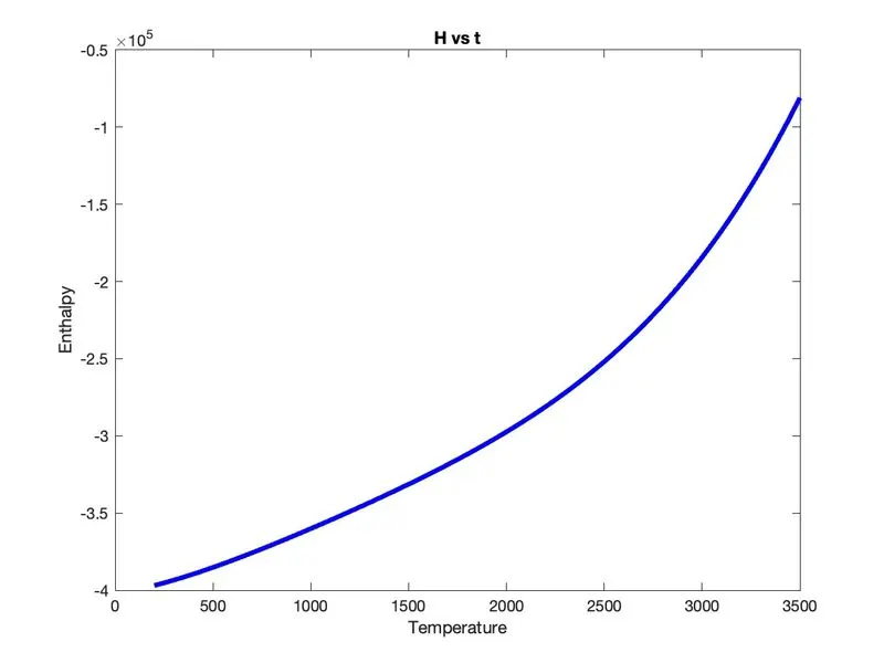
- Plot the Cp, Enthalpy and Entropy for the local temperature range (low temperature : high temperature) specific for each species.
- Save the plots as images with appropriate names and dump them in separate folders for each species with suitable name. All these should be generated automatically.
- The main program should just take the "THERMO.dat" file as an input and generate Cp, H and S plots.
- Plots for o2, N2 and Co2 species
THEORY
Parsing of data : It is the process of reading of external data from a data file or writting a data into an external data file using fopen('name of datafile', 'r') command for reading from the data file and fopen('name of datafile', 'w') for writting into the data file.
NASA Thermodynamic data: NASA came up with polynomials that can be used to evaluate thermodynamic properties such as Cp, H and S. They have also documented the co-efficients that are required to evaluate these polynomials for 1000+ species.
Specific heat Cp :It is the quantity of heat required to raise the temperature of one gram of a substance by one Celsius degree.
Enthalpy H:It is a property of a thermodynamic system, which is the sum of the system's internal energy and the product of its pressure and volume. Equation of enthalpy is
- H = U + pV, where U is the internal energy, p is pressure, and V is the volume of the system.
Entropy S: Entropy is a scientific concept as well as a measurable physical property that is most commonly associated with a state of disorder, randomness, or uncertainty.
EQUATIONS USED
Specific Heat Cp = R*(a1+a2*(t)+a3*(t.^2)+a4*(t.^3)+a5*(t.^4))
Enthalpy H =R*t(a1+a2*(t./2)+a3*((t.^2)./3)+a4*((t.^3)./4)+a5*((t.^4)./5)+a6./t)
Entropy S =R*(a1*log(t)+a2.*t+a3*((t.^2)./2)+a4*((t.^3)./3)+a5*((t.^4)./4)+a7)
Here R is the universal gas constant
BODY OF CONTENT
- The first step of the program is to open the data file THERMO.dat and read it using the f1 = fopen('THERMO.dat','r') command.
clear all
close all
clc
%input
R = 8.314
%Reading the file from THERMO,dat
f1 = fopen('THERMO.dat','r')
%Skipping the first 5 lines using fgetl
for i = 1:5
fgetl(f1)
end- Then we need to skip the next 5 steps which are just the comments given in the data file , for that we use the fgetl command and put it inside a for loop. The fgetl command should be followed by the file f1 which we opened early. Then we end the loop using END command
- The next step is to calculate the local low temperature ,local mid temperature and local high temperature
for j = 1:53

tline = fgetl(f1)
A = strsplit(tline,' ')
z = length(A)
species = A{1}
%local temperatures
lower_temp = str2double(A{z-3})
mid_temp = str2double(A{z-1})
higher_temp = str2double(A{z-2})
t = linspace(lower_temp,higher_temp,500)- For this first we need to get on to the line where the data is present , thus we use fgetl command and assign a variable called tline to it.
- Then we split the string which is obtained by executing the fgetl command. It is done to extract the useful datas from the string using the stringsplit command. In strsplit command the string tline is splitted at points where space is present, which is given as the command. It is then assigned to a variable 'A' for further use.
- Then a variable z is assigned to the length of A. Then the first cell of A is assigned as species , because it is the array which stores all the species names.
Now we find lower local temperature , mid local temperature and higher local temperature using str2double command , which converts the above string into the number and the position of the numbers(i.e. temperatures) which is to be converted is determined by inputting the position where the temperature values are present. It is carried out using the following command
- The next step is to calculate the coefficients of higher temperature and lower temperature for that the program is carried out in the following manner. Here a1 to a7 is high temperature coefficients and a8 to a14 is low temperature coefficients
%High temperature coefficients

tline1 = fgetl(f1);
a = findstr(tline1,'E');
a1 = tline1(1:a(1)+3);
a1 = str2double(a1);
a2 = tline1(a(1)+4:a(2)+3);
a2 = str2double(a2);
a3 = tline1(a(2)+4:a(3)+3);
a3 = str2double(a3);
a4 = tline1(a(3)+4:a(4)+3);
a4 = str2double(a4);
a5 = tline1(a(4)+4:a(5)+3);
a5 = str2double(a5);

tline2 = fgetl(f1);

b = findstr(tline2,'E');
a6 = tline2(1:b(1)+3);
a6 = str2double(a6);
a7 = tline2(b(1)+4:b(2)+3);
a7 = str2double(a7);

%Lower temperature coefficients

a8 = tline2(b(2)+4:b(3)+3);
a8 = str2double(a8);
a9 = tline2(b(3)+4:b(4)+3);
a9 = str2double(a9);
a10 = tline2(b(4)+4:b(5)+3);
a10 = str2double(a10);

tline3 = fgetl(f1);
c = findstr(tline3,'E');
a11 = tline3(1:c(1)+3);
a11 = str2double(a11);
a12 = tline3(c(1)+4:c(2)+3);
a12 = str2double(a12);
a13 = tline3(c(2)+4:c(3)+3);
a13 = str2double(a13);
a14 = tline3(c(3)+4:c(4)+3);
a14 = str2double(a14);- At first we get to the line whose coefficients are to be found for that we use the fgetl command and we assign a variable tline1 to it.
- Then we find the string and seperate it at the point where E is present for calculating the specific coefficent of that string using the command findstr(tline1,'E') also we assign a variable 'a' to the command
- After executing this command we will be getting a string with required value and then we calculate the coefficient of the whole string using the command
- a1 = tline1(1:a(1)+3); which results in the following output 2.56942078E+00 . This command is used to display the first value from the string to the value where the E is present (that is shown as a(1)) and then 3 more places are added so that the output comes as shown above
- Then we convert this string into numerical value using the str2double command , where conversion into double helps in getting more accurate values
- The next step is to calculate a2 the only difference is that in the command to calculate a2 , i.e. a2 = tline(a(1)+4:a(2)+3) here a(1)+4 is the position where the second string starts and a(2)+3 is the end position of the second string and then the conversion of string to double takes place
- This method is carried out through out the process upto a5 and then we need to jump into the next line for that we again use fgetl command and assign a variable tline2 to it. Then the same procedure is followed till the a7.
- After a7 we calculate the lower temperature coefficients upto a14 with the same procedure. Also after a10 we jump into the next line using fgetl command and assigning a variable tline3 to it.
- The next step is to calculate Specific heat Cp , Enthalpy H, Entropy S and Molecular weight using function definitions and by calling those functions
function [H] = enthalpy_func(a1,a2,a3,a4,a5,a6,a8,a9,a10,a11,a12,a13,t,R,mid_temp)
if t>= mid_temp
    H = R*t.*(a1+a2*(t./2)+a3*((t.^2)./3)+a4*((t.^3)./4)+a5*((t.^4)./5)+a6./t);
else
    H =  R*t.*(a8+a9*(t./2)+a10*((t.^2)./3)+a11*((t.^3)./4)+a12*((t.^4)./5)+a13./t);
end
end
In the above function the enthalpy H is calculated by defining the function enthalpy_func with the input values a1,a2,a3,a4,a5,a6,a8,a9,a10,a11,a12,a13,t,R,mid_temp
mid_temp is the middle/medium temperature which we calculated early
If the temperature t is greater than the mid_temp then we use the equation. This is carried out using the if command and else command.
function [S] = entropy_func(a1,a2,a3,a4,a5,a7,a8,a9,a10,a11,a12,a14,mid_temp,R,t)
if t >= mid_temp
    S = R*(a1*log(t)+a2.*t+a3*((t.^2)./2)+a4*((t.^3)./3)+a5*((t.^4)./4)+a7);
else
     S = R*(a8*log(t)+a9.*t+a10*((t.^2)./2)+a11*((t.^3)./3)+a12*((t.^4)./4)+a14);
end- Now we find entropy using the function entropy_func with input values a1,a2,a3,a4,a5,a7,a8,a9,a10,a11,a12,a14,t,R,mid_temp
- Similar to the enthalpy function here also we use the if command and check whether t>= mid_temp , if so we use the following equation to calculate entropy S
- Then we calculate Specific heat by defining the function specific_heat_func with the input values a1,a2,a3,a4,a5,a8,a9,a10,a11,a12,t,R,mid_temp
function [Cp] = specific_heat_func(a1,a2,a3,a4,a5,a8,a9,a10,a11,a12,t,R,mid_temp)
if t>= mid_temp
    Cp = a1+a2*(t)+a3*(t.^2)+a4*(t.^3)+a5*(t.^4);
else
       Cp = a8+a9*(t)+a10*(t.^2)+a11*(t.^3)+a12*(t.^4);
end

end
Here we calculate Specific Heat using the equation
- Now we calculate the molecular weight of all the species as per reqiuirement by defining the function molecular_weight with input values as species.
function [mol_weight] = molecular_weight(species)
%defining elements
element = ['O','C','H','N','A'];
fprintf('Molecular Weight of ')
fprintf(species)
fprintf(' : ' )
%atomic weight of the elements
atomic_weight =  [16,12,1,14,39];
mol_weight = 0;
for i =1:length(species)
    for j = 1:length(element)

    if strcmp(species(i),element(j))

   mol_weight = mol_weight+atomic_weight(j);
        p = j;
    end

    end
     n = str2num(species(i));

if n>1
    mol_weight = mol_weight+atomic_weight(p)*(n-1);
end
end
fprintf('Molecular Weight of %s :',species)
fprintf('%d',mol_weight)
disp(' ')
end
Here first we define the elements which are the basic elements of the species present and store it in an array called 'element'.
Then we print the lines 'Molecular Weight of' species ':' using the fprintf command where the species are all the species whose molecular weight is to be found.
The next step is to define the atomic weight of the elements defined, for that cerate an array called atomic_weight and store the atomic weights of respective elements.
Then we put initial molecular weight of the species as 0 and this is done to initiate the process of calculation of molecular weight
After that we create two for loops i and j of which i varies from 0 to the length of species i.e. 53 and j loop varies from 0 to length of elements which is 5. This is done to compare the species with elements and also calculate the molecular weight using the equation mol_weight = mol_weight+atomic_weight(j);
We store the value of j into a variable p then we end both the commands and calculate 'n' which is the number of species present in a molecule for eg. in co2 there is one mole of carbon and 2 moles of oxygen thus to calculate the molecular weight we have to add these 2 moles of oxygen which makes it 16*2= 32 . Here 2 is the 'n'. Similarly for other species the molecular weight is calculated using the n whose value is always greater than 1. For those species we calculate the molecular weight using the below equation
In the above equation the molecular weight of co2 will turn out to be (12+16)+16*(2-1) = 44
similarly for CH4 (12+1)+1*(4-1) = 16
Now we end the if command and the loop using the end command and write the command to print 'Molecular weight of ' species ':' and to print the molecular weight using the fprintf command. Here %s is to show it is a string and %d is used to show that molecular weight is a double. Then we need to display the molecular weights of all the species thus we use the disp command.
- Now we call the functions of Enthalpy, Entropy, Specific Heat and Molecular weight so that we could calculate them.
%Calculating specific heat Cp
Cp = specific_heat_func(a1,a2,a3,a4,a5,a8,a9,a10,a11,a12,t,R,mid_temp) ;
%Calculating enthalpy H
H = enthalpy_func(a1,a2,a3,a4,a5,a6,a8,a9,a10,a11,a12,a13,t,R,mid_temp);
%Calculating Entropy S
S =  entropy_func(a1,a2,a3,a4,a5,a7,a8,a9,a10,a11,a12,a14,mid_temp,R,t);
%calculating molecular weight
[mol_weight] = molecular_weight(species)- Now we have to plot and save the program for that we craeate a program as shown below
-
%plotting Cp vs t mkdir(['/Users/aadarshr/Documents/Aadarsh/',species]) figure(1) plot(t,Cp,'linewidth',3,'color','r') title('Cp vs t') xlabel('Temperature') ylabel('Specific Heat') %plotting S vs t figure(2) plot(t,S,'linewidth',3,'color','y') xlabel('Temperature') ylabel('Entropy') title('S vs t') %plotting H vs t figure(3) plot(t,H,'linewidth',3,'color','b') xlabel('Temperature') ylabel('Enthalpy') title('H vs t') cd(['/Users/aadarshr/Documents/Aadarsh/',species]) saveas(1,'Cp vs t','jpg') saveas(2,'H vs t','jpg') saveas(3,'S vs t','jpg') cd(['/Users/aadarshr/Documents/']) end - In the above program at first we create a directory named '/Users/aadarshr/Documents/Aadarsh/' using mkdir command, this command makes a directory with plots of all the species and assigns the address that is given by us.
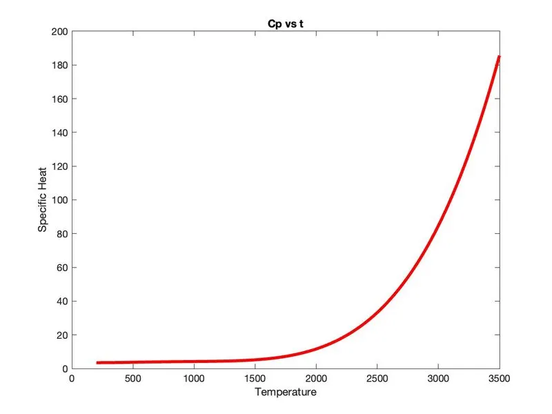
- Then we plot Specific heat vs temperature using plot command with x axis as temperature and y axis labelled as Specific heat. We also plot the Enthalpy vs Temperature and Entropy vs Temperature in the similar manner. Exception is that the y axis will be labelled as H and S respectively.
- Then we change the directory using cd command and save the plots of the species in jpg format using the saveas command
- At last we end the j loop using END command
OUTPUT
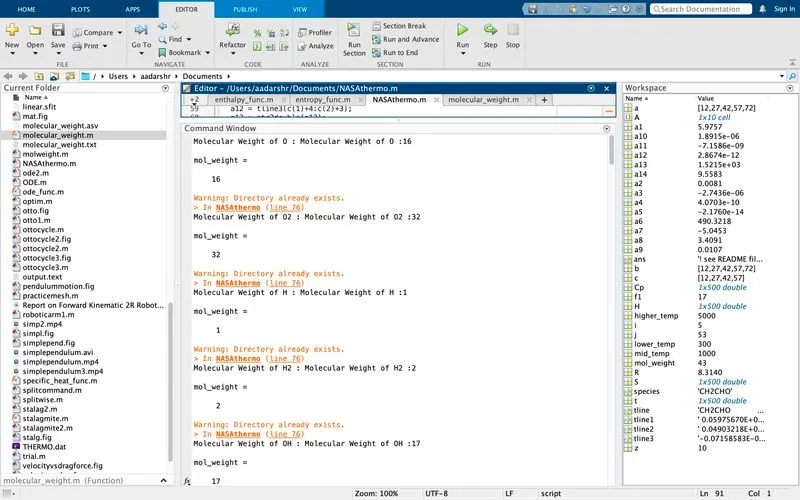
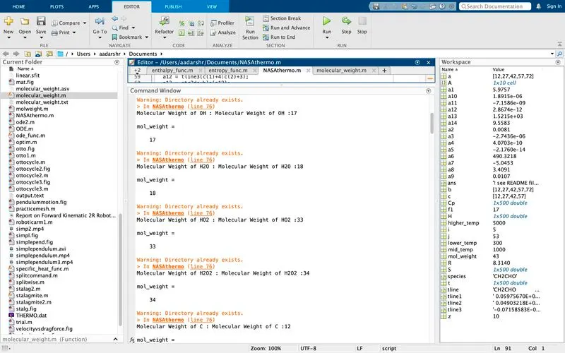
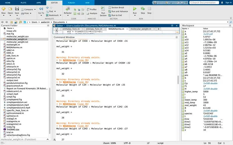
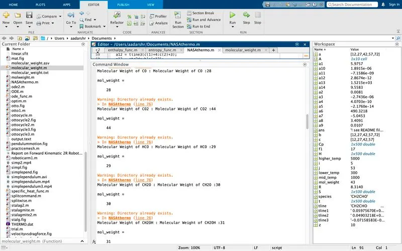
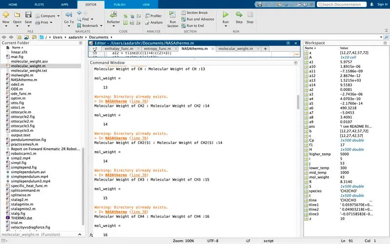
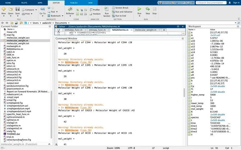
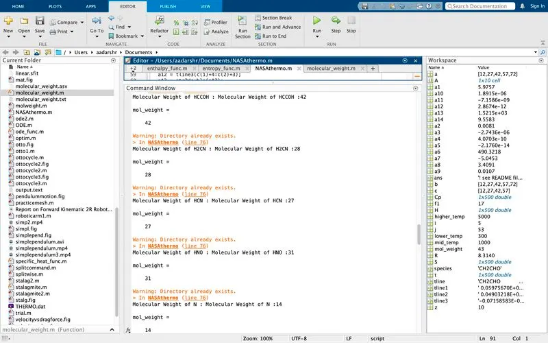
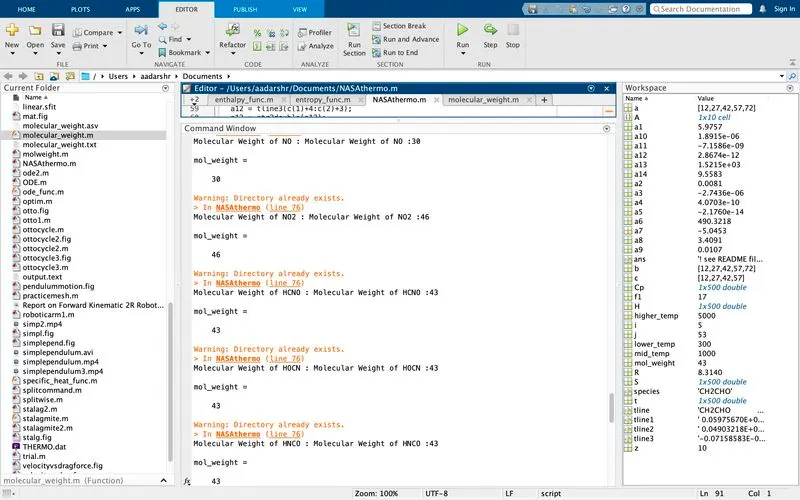
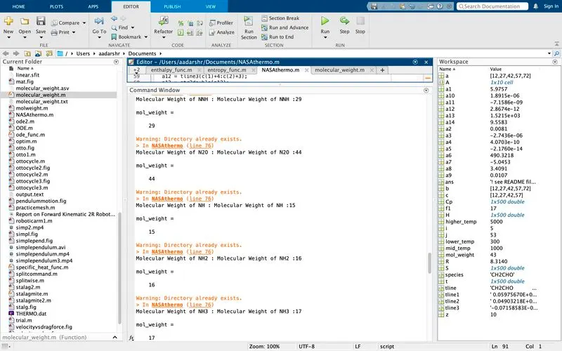
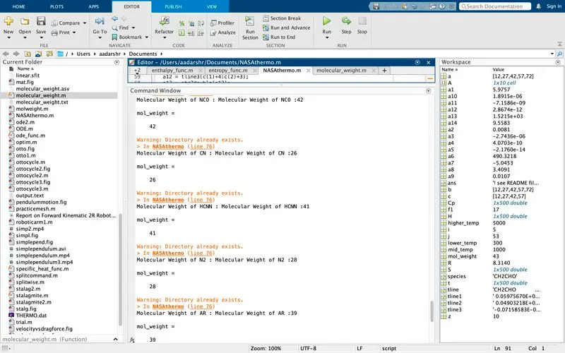
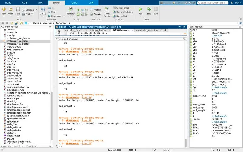
Output showing the molecular weight of each species is as follows
Screenshot of the window were all folders are saved

Plots of o2
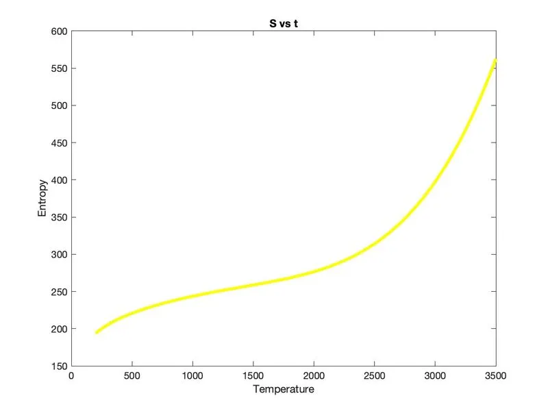
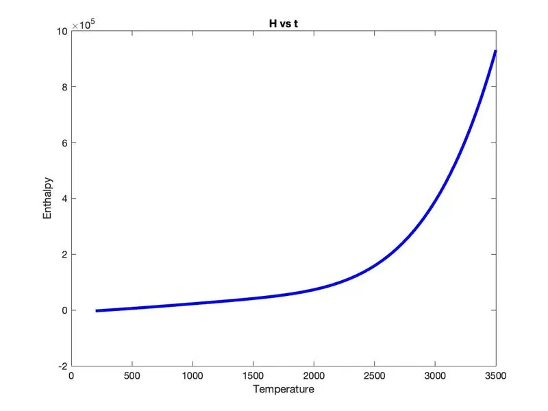
Plots of N2
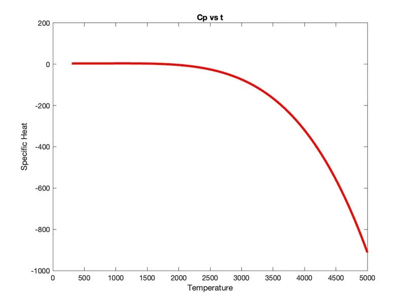
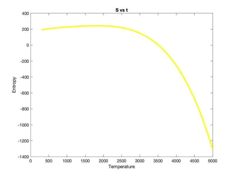
Plots of Co2
ERRORS OCCURED
Forgot to use the dot product while multiplying a matrix i.e here 't' in the specific heat function ,thus the following error message popped up.
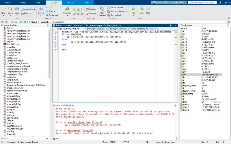
it is done because the matrix is square and the power is a scalar quatity , for scalar multiplicaation/division dot product is necessary.
Thus we put the dot and after putting the dot the function got defined and it is called in the main program and the program got executed.
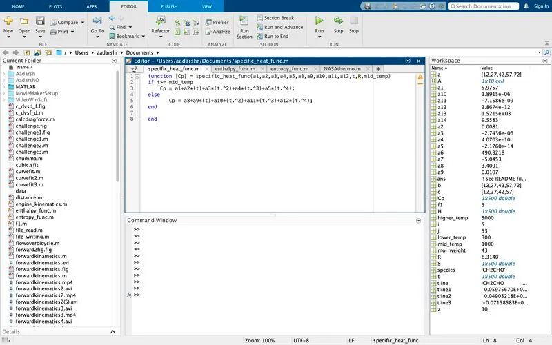
- Forgot to put END command at the last of the main program which resulted in the popping of the following message.
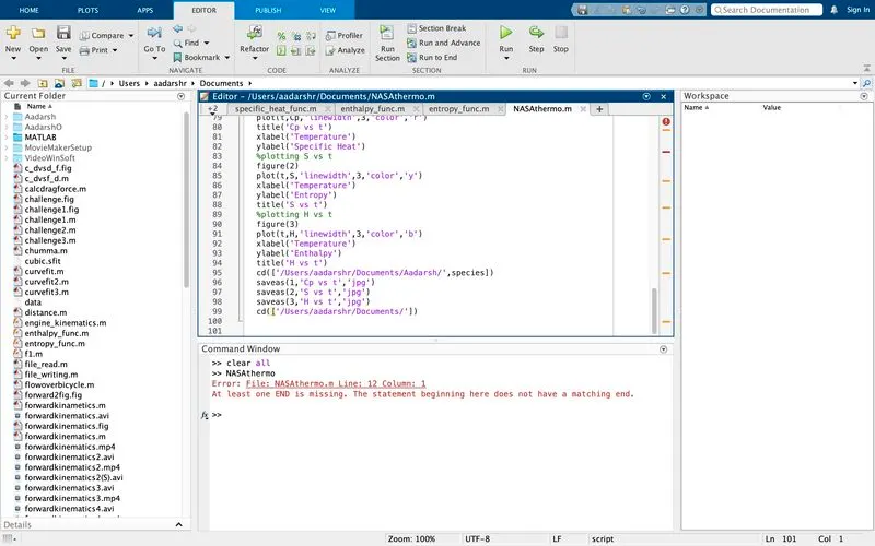
After putting END command the program got executed
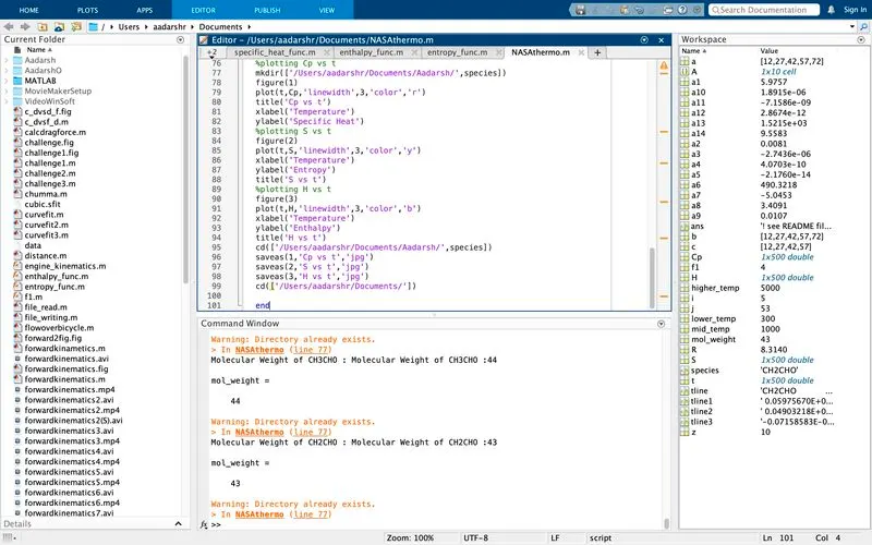
RESULT
The molecular weight of o2 = 32
molecular weight of Co2 = 44
molecular weight of N2 = 28
The rest of the molecular weights are displayed on the command window
CONCLUSION
The program to parse the NASA Thermodynamic data and to calculate the molecular weight of the species present inside the data and also to display it in the command window is successfully carried out and the results are noted down along with the plots.
REFERENCES
MATHWORKS, Google, Wikipedia,