Challenge

Project 2 - Rankine cycle Simulator

AAadarsh R2 Jun 2022

MATLAB

A program to create a Rankine Cycle Simulator

AIM

To write a program that creates a Rankine Cycle Simulator

OBJECTIVE

Create a Rankine Cycle Simulator using OCTAVE/MATLAB.
The code should calculate the state points of the Rankine Cycle based on user inputs.
Then, plot the corresponding T-s and h-s plots for the given set of inputs.

EQUATIONS USED

x2 = ((s2 - sf2)/(sg2-sf2));

h2 = hf2+x2*(hg2 - hf2);

where x2 is the dryness fraction at point 2, h2 and s2 are the enthalpy and entropy at pont 2 , sf2 and hf2 are the entropy and enthalpy at liquid state along the liquid saturation line and sg2 and hg2 are the entropy and enthalpy at vapour saturaion line.

k = Cp4/Cv4;

t4 = t3/((p3/p4)^((k-1)/k));

Here k is the heat capacity ratio and this ratio is used to calculate t4 which is the temperature at point 4 and t3 and p3 are temperature and pressure at point3

wt = h1-h2;

It is the turbine work generated by the turbine

wp = v3*(p4 - p3);

It is the input work done on the pump to compress the steam

Qin = h1 - h4;

Heat given into the system by the boiler

Qout = h2 - h3;

heat generated out of the system by the condenser

Ntherm = (wt - wp)/Qin;

Thermal efficiency which is the ratio of net work and heat supplied to the system

BWratio = wp/wt;

Back work ratio which is the ratio of pump work to turbine work

ssc = 3600/(wt-wp) Kg/KWh;

ssc is the specific steam consumption which is the amount of steam cosumed per unit of power produced in KW

wnet = wt - wp;

Net work created is the required work output which is the difference between turbine work and pump work

THEORY

Rankine Cycle

It is the working cycle of steam turbine / steam power plant. It consists of mainly 4 processes

Isentropic Expansion : Expansion of steam coming from boiler isentropically by the Turbine
Constatnt Pressure Heat Rejection : Heat rejection at constant pressure by the condenser to the surroundings
Isentropic Compression : Compression of the steam isentropically by the pump
Constant Pressure Heat Addition : Heat is added to the system by the boiler at constant pressure.

The components used in rankine cycle are:-

Turbine : Turbine is used to expand the steam isentropically and it is connected to a generator which generates electricity from the rotation of the turbine
Condenser : It is used to condense the steam that comes from the Turbine by circulating water and rejecting the heat to the surroundings.
Pump : It is the device used to compress the condensed steam coming from the condenser and this process is carried out isentropically
Boiler : Boiler is used to boil the steam coming from the pump. The steam is heated into a superheated state for acquiring greater efficiency. This steam is circulated back into the Turbine for work generation and all the 4 processes continues in a cyclic manner.

The above shown process is the basic working cycle of steam power plant.

BODY OF CONTENT

clear all
close all
clc

%A program to create a Rankine Cycle Simulator

%input variables
p1 = 30;
t1 = 400;
p2 = 0.05;
%state points for state 1
h1 = XSteam('h_pt',p1,t1);
s1 = XSteam('s_pt',p1,t1);
s2 = s1;
%state points at state 2

hf2 = XSteam('hL_p',p2);
hg2 = XSteam('hV_p',p2);
sf2 = XSteam('sL_p',p2);
sg2 = XSteam('sV_p',p2);
x2 = ((s2 - sf2)/(sg2-sf2));
h2 = hf2+x2*(hg2 - hf2);
t2 = XSteam('T_ph',p2,h2);

%state points at state 3

p3 = p2;
t3 = t2;
h3 = XSteam('hL_p',p3);
s3 = XSteam('sL_p',p3);
v3 = XSteam('vL_p',p3);
%state points at state 4
p4 = p1;
s4 = s3;
Cp4 = XSteam('Cp_ps',p4,s4);
Cv4 = XSteam('Cv_ps',p4,s4);
k = Cp4/Cv4;
t4 = t3/((p3/p4)^((k-1)/k));
h4 = XSteam('h_ps',p4,s4);


%state points at state 5 
t6 = XSteam('Tsat_p',p4);
t5 = t6;
h5 = XSteam('hL_p',p4);
h6 = XSteam('hV_p',p4);
s5 = XSteam('sL_p',p4);
s6 = XSteam('sV_p',p4);

The first step of the program is to input the given values of p1,t1,p2 and after that we will begin to define the state points for each state

For that we use the data file XSteam which has the various properties of liquids and gaseous like enthalpy, entropy, specific heat, pressure, etc. We find the enthalpy and entropy at point 1 using the below command

h1 = XSteam('h_pt',p1,t1);

s1 = XSteam('s_pt',p1,t1);

In this command h_pt and s_pt are the enthalpy and entropy as a function of pressure and temperature which is used to find the values of h1 and s1 at pressure p1 and temperature t1.

Since the first process is an isentropic process(isentropic expansion from 1-2) s2 = s1

Then we calculate the state points at the second state for doing that first we have to calculate the enthalpy and entropy of steam at liquid state and at vapour state seperately. Thus we use the following equation

hf2 = XSteam('hL_p',p2);

hg2 = XSteam('hV_p',p2);

sf2 = XSteam('sL_p',p2);

sg2 = XSteam('sV_p',p2);

where sf2 and sg2 are the entropy of liquid and gas at saturation curve and hf2 and hg2 are the enthalpy of liquid state and gaseous state at saturation curve. They are found out by using the XSteam data file and taking the value of enthalpy of liquid as a function of pressure at pressure p2 and for vapour phase hV_p is used at p2 pressure.

Similarly entropy at liquid and vapour phase along the saturation curve is found out using these equations at the pressure p2

sf2 = XSteam('sL_p',p2);

sg2 = XSteam('sV_p',p2); where sV_p and sL_p are the entropy along the vapour and liquid curves as a function of pressure p2

Next stage is to calculate x2 which is necessary to calculate h2 using the equation x2 = ((s2 - sf2)/(sg2-sf2)); where x2 is the dryness fraction at point 2.

After calculating we calculate h2 and using the value of h2 we find the value of temperature t2 using the equation

t2 = XSteam('T_ph',p2,h2);

Here 'T_ph' is the temperature as a function of pressure and enthalpy at pressure p2 and enthalpy h2 is used to calculate t2 using the XSteam data file.

Similarly the state points at state 3 is found out. Here since it is a constant pressure heat rejection process p3 = p2 and from the T S diagram we can find that t3 = t2

h3 , s3 and v3 i.e enthalpy , entropy and volume at state 3 is calculated from the XSteam data file and using the value of hL_p, sL_p and vL_p. It is used because the state 3 lies on the liquid saturation curve and we calculate those values as a function of pressure p3. We calculate v3 to find the pump work/ input work later in the programThe command is as follows

h3 = XSteam('hL_p',p3);

s3 = XSteam('sL_p',p3);

v3 = XSteam('vL_p',p3);

The next stage is to define the state points 4, here we calculate specific heat at constant volume Cv and specific heat at constant pressure Cp. It is used to calculate t4 where t4 is the temperature at state 4 i.e. after isentropic compression of steam and the point lies above the liquid saturation line, thus we require to use Cp and Cv to calculate t4

k = Cp4/Cv4;

t4 = t3/((p3/p4)^((k-1)/k));

Here k is the heat capacity ratio and this ratio is used to calculate t4 which is the temperature at point 4 and t3 and p3 are temperature and pressure at point3

Also we calculate h4 using enthalpy as a function of pressure and entropy p4 and s4

here since the process 4 - 1 is constant pressure heat addition process p4 = p1 and process 3 - 4 is isentropic compression s4 = s3

Now we find the state point at 5 and 6 where t6 is calculated using the XSteam data file and taking the value of Tsat_p i.e saturation temperature as a function of pressure p4.

Since state point 6 lies in the vapour saturation curve thus we calculate h6 and s6 on the basis of that i.e. for h6 'hV_p' at p4 is calculated and for s6 'sV_p' at p4 is calculated

similarly h5 and s5 is calculated using 'hL_p' and 'sL_p' at pressure p4, because state point 5 lies in the saturated liquid region

%calculating output values
wt = h1-h2;
wp = v3*(p4 - p3);
Qin = h1 - h4;
Qout = h2 - h3;
Ntherm = ((wt - wp)/Qin)*100;
BWratio = wp/wt;
ssc = 3600/(wt-wp);
wnet = wt - wp;

The next step is to calculate the output values , first we calculate the turbine work which is the work generated by the turbine due to the rotation of blades and the blades are connected to a shaft which is connected to a generator which generates electricity

wt = h1-h2;

It is the turbine work generated by the turbine, it is the difference in the enthalpy ar point1 and point2 i.e. enthalpies at isentropic expansion process

wp = v3*(p4 - p3);

It is the input work done on the pump to compress the steam. Here pump work is the product of volume before compression i.e. v3 and the difference in pressure before compression and after compression i.e p4-p3

Qin = h1 - h4;

Heat given into the system by the boiler

Qout = h2 - h3;

heat generated out of the system by the condenser

Ntherm = ((wt - wp)/Qin)*100;

Thermal efficiency which is the ratio of net work and heat supplied to the system

BWratio = wp/wt;

Back work ratio which is the ratio of pump work to turbine work

ssc = 3600/(wt-wp) Kg/KWh;

ssc is the specific steam consumption which is the amount of steam cosumed per unit of power produced in KW

wnet = wt - wp;

Net work created is the required work output which is the difference between turbine work and pump work

%Calculating the points on the saturation curves
T=linspace(1,400,1000);
for i=1:length(T)
sf(i)=XSteam('sL_T',T(i));
sg(i)=XSteam('sV_T',T(i));
hf(i)=XSteam('hL_T',T(i));
hg(i)=XSteam('hV_T',T(i));
end
%plotting
subplot(1,2,1);
%plotting T-S Curve
plot(sf,T,'color','b');
hold on
plot(sg,T,'color','r');
%plotting T-S diagram
plot([s1 s2],[t1 t2],[s2 s3],[t2 t3],[s3 s4],[t3 t4],[s4 s5],[t4 t5],[s5 s6],[t5 t6],[s6 s1],[t6 t1],'linewidth',1,'color','k');
legend('staurated liquid','saturated vapour')
%Texting the points
text(s1,t1,'1','color','r');
text(s2,t2,'2','color','r');
text(s3,t3-5,'3','color','r');
text(s4,t4+10,'4','color','r');
text(s5,t5,'5','color','r');
text(s6,t6,'6','color','r');
%labelling
xlabel('Entropy');
ylabel('Temperature');
title('T-S Diagram')
axis([0 10 0 500]);
% plotting H-S diagram

subplot(1,2,2);
plot([s1 s2],[h1 h2],'linewidth',1,'color','k');
hold on
plot([s2 s3],[h2 h3],'linewidth',1,'color','k');
plot([s3 s4],[h3 h4],'linewidth',1,'color','k');
plot([s4 s5],[h4 h5],'linewidth',1,'color','k');
plot([s5 s6],[h5 h6],'linewidth',1,'color','k');
plot([s6 s1],[h6 h1],'linewidth',1,'color','k');

%labelling
xlabel('Entropy');
ylabel('Enthalpy');
title('H-S Diagram')
%plotting H-S curve
plot(sg,hg,'color','r');
plot(sf,hf,'color','b');
%Texting the points 
text(s1,h1,'1','color','r');
text(s2,h2,'2','color','r');
text(s3,h3-60,'3','color','r');
text(s4,h4+160,'4','color','r');

Next step is to calculate the state points on the saturation curve

First we have to create an array T that stores the value of temperature variying from 1 to 400 with an interval of 1000 values in between them using the linspace command.

Now we have to use a for loop 'i' that varies from 1 to length of T i.e. 1000 so that the values of entropy and enthalpy through the saturated liquid and saturated vapour line can be found out for each value of 'i'. For that the following command is used

for i=1:length(T)

sf(i)=XSteam('sL_T',T(i));

sg(i)=XSteam('sV_T',T(i));

hf(i)=XSteam('hL_T',T(i));

hg(i)=XSteam('hV_T',T(i));

end

Here sL_T ,sV_T are the saturated liquid and vapour entropy values as a function of temperature T(i) which is used to calcullate sf(i) and sg(i), similarly hL_T and hV_T are the saturated liquid and vapour enthalpy values as a function of temperature T(i) which is used to calcullate hf(i) and hg(i). Then we end the loop using END command

The next step is to plot the T-S saturation curve , for that first we create a subplot using subplot command which consists of 2 columns and 1 row so the command is given as follows

subplot(1,2,1);

Then we plot the T-S curve using the plot command and with sf and T as x and y values then after using the hold on command to keep the first plot unerased and then we create the second plot of saturated vapour curve with sg and T as input values

Now we plot the T-S diagram of the Rankine Cycle using the plot command and we give s1 to s6 and t1 to t6 as the x and y input values. The command is as follows

plot([s1 s2],[t1 t2],[s2 s3],[t2 t3],[s3 s4],[t3 t4],[s4 s5],[t4 t5],[s5 s6],[t5 t6],[s6 s1],[t6 t1],'linewidth',1,'color','k');

We also use the legend command to distinguish the saturated liquid curve and saturated vapour curve where 'saturated liquid curve' is given in blue colour and 'saturated vapour curve' is given in red colour.

Then texting of the points for the plot is given using text command. Here in the below given command t3-5 and t4+10 is used to make the texts at point 3 and 4 more legible

text(s3,t3-5,'3','color','r');

text(s4,t4+10,'4','color','r');

Next step is to label the plot using label command as x axis is labelled as Entropy and y axis is labelled as Temperature and also a fixed axis is given to make the plot more clear where the x axis varies from 0 to 10 and y axis varies from 0 to 500

Similarly we plot the H-S diagram and H-S curve only difference is that we label y axis as Enthalpy and plot the values of enthalpy against entropy. This plot is plotted on the second column that was created early using the subplot command. Then we plot the points on the plot using the text command

%printing the process details
fprintf('\n                              RANKINE CYCLE SIMULATOR                    \n\n')
fprintf('1 - 2 is Isentropic Expansion in the Turbine\n')
fprintf('2 - 3 is Constant Pressure Heat Rejection by the Condenser\n')
fprintf('3 - 4 is Isentropic Compression in the Pump\n')
fprintf('4 - 1 is Constant Pressure Heat Addition by the Boiler\n')
fprintf('\n')
fprintf('Enter the Pressure at the Turbine inlet(in bar) :  30\n')
fprintf('Enter the Temperature at the Turbine inlet (in Degree Celcius) :  400\n')
fprintf('Enter the Pressure at Condense inlet (in bar) :  0.05\n')
fprintf('                                 RESULTS                \n')



%Description at State1
fprintf('At State Point 1 :\n')
fprintf('p1 is : 30 Bar\n')
fprintf('t1 is : 400 Degree celcius\n')
fprintf('h1 is : 3.231571027259653e+03 KJ/Kg\n')
fprintf('s1 is : 6.9233 KJ/Kg K\n\n')

%Description at State2
fprintf('At state point 2 :\n')
fprintf('p2 is : 0.05 Bar\n')
fprintf('t2 is : 32.875 Degree celcius\n')
fprintf('h2 is : 2.110708212003693e+03 KJ/Kg\n')
fprintf('x2 is : 0.8143\n')
fprintf('s2 is : 6.9233 KJ/Kg K\n\n')

%Description at State3
fprintf('At state point 3 :\n')
fprintf('p3 is : 0.05 Bar\n')
fprintf('t3 is : 32.875 Degree celcius\n')
fprintf('h3 is : 137.7651 KJ/Kg\n')
fprintf('s3 is : 0.4763 KJ/Kg K\n\n')

%Description at State4
fprintf('At state point 4 :\n')
fprintf('p4 is : 30 Bar\n')
fprintf('t4 is : 36.9353 Degree celcius\n')
fprintf('h4 is : 140.7622 KJ/Kg\n')
fprintf('s4 is : 0.4763 KJ/Kg K\n\n')

%Other required output datas 
fprintf('wt is : 1.120862815255960e+03 KJ/Kg\n')
fprintf('wp is : 0.0301 KJ/Kg\n')
fprintf('wnet is : 1.120832705885940e+03 KJ/Kg\n')
fprintf('Ntherm is : 36.26 percent \n')
fprintf('ssc is : 3.2119 Kg/KWh \n')
fprintf('Bw ratio is : 2.6863e-05 \n')

The last step of the program is to print the detailes or description of the values obtained as required in the command window. Inorder to display the required detailes in the command window we use the fprintf command which prints the comments that is written inside the command enclosed in single quotes. The command is as shown :

fprintf('At State Point 1 :\n') This command prints the line 'At State point 1 :' in the command window and \n is used to print the next line below it. Without \n all the lines or descriptions printed will be in a straight line. For eg if we print fprintf('At State Point 1:') and then print fprintf('p1 is : 30 bar') without \n the output obtained will be At State point 1 : p1 is : 30 bar

If we put \n in it then the output will be

At State Point 1 :

p1 is : 30 bar

MAIN PROGRAM

clear all
close all
clc

%A program to create a Rankine Cycle Simulator

%input variables
p1 = 30;
t1 = 400;
p2 = 0.05;
%state points for state 1
h1 = XSteam('h_pt',p1,t1);
s1 = XSteam('s_pt',p1,t1);
s2 = s1;
%state points at state 2

hf2 = XSteam('hL_p',p2);
hg2 = XSteam('hV_p',p2);
sf2 = XSteam('sL_p',p2);
sg2 = XSteam('sV_p',p2);
x2 = ((s2 - sf2)/(sg2-sf2));
h2 = hf2+x2*(hg2 - hf2);
t2 = XSteam('T_ph',p2,h2);

%state points at state 3

p3 = p2;
t3 = t2;
h3 = XSteam('hL_p',p3);
s3 = XSteam('sL_p',p3);
v3 = XSteam('vL_p',p3);
%state points at state 4
p4 = p1;
s4 = s3;
Cp4 = XSteam('Cp_ps',p4,s4);
Cv4 = XSteam('Cv_ps',p4,s4);
k = Cp4/Cv4;
t4 = t3/((p3/p4)^((k-1)/k));
h4 = XSteam('h_ps',p4,s4);


%state points at state 5 
t6 = XSteam('Tsat_p',p4);
t5 = t6;
h5 = XSteam('hL_p',p4);
h6 = XSteam('hV_p',p4);
s5 = XSteam('sL_p',p4);
s6 = XSteam('sV_p',p4);

%calculating output values
wt = h1-h2;
wp = v3*(p4 - p3);
Qin = h1 - h4;
Qout = h2 - h3;
Ntherm = ((wt - wp)/Qin)*100;
BWratio = wp/wt;
ssc = 3600/(wt-wp);
wnet = wt - wp;

%Calculating the points on the saturation curves
T=linspace(1,400,1000);
for i=1:length(T)
sf(i)=XSteam('sL_T',T(i));
sg(i)=XSteam('sV_T',T(i));
hf(i)=XSteam('hL_T',T(i));
hg(i)=XSteam('hV_T',T(i));
end
%plotting
subplot(1,2,1);
%plotting T-S Curve
plot(sf,T,'color','b');
hold on
plot(sg,T,'color','r');
%plotting T-S diagram
plot([s1 s2],[t1 t2],[s2 s3],[t2 t3],[s3 s4],[t3 t4],[s4 s5],[t4 t5],[s5 s6],[t5 t6],[s6 s1],[t6 t1],'linewidth',1,'color','k');
legend('staurated liquid','saturated vapour')
%Texting the points
text(s1,t1,'1','color','r');
text(s2,t2,'2','color','r');
text(s3,t3-5,'3','color','r');
text(s4,t4+10,'4','color','r');
text(s5,t5,'5','color','r');
text(s6,t6,'6','color','r');
%labelling
xlabel('Entropy');
ylabel('Temperature');
title('T-S Diagram')
axis([0 10 0 500]);
% plotting H-S diagram

subplot(1,2,2);
plot([s1 s2],[h1 h2],'linewidth',1,'color','k');
hold on
plot([s2 s3],[h2 h3],'linewidth',1,'color','k');
plot([s3 s4],[h3 h4],'linewidth',1,'color','k');
plot([s4 s5],[h4 h5],'linewidth',1,'color','k');
plot([s5 s6],[h5 h6],'linewidth',1,'color','k');
plot([s6 s1],[h6 h1],'linewidth',1,'color','k');

%labelling
xlabel('Entropy');
ylabel('Enthalpy');
title('H-S Diagram')
%plotting H-S curve
plot(sg,hg,'color','r');
plot(sf,hf,'color','b');
%Texting the points 
text(s1,h1,'1','color','r');
text(s2,h2,'2','color','r');
text(s3,h3-60,'3','color','r');
text(s4,h4+160,'4','color','r');

%printing the process details
fprintf('\n                              RANKINE CYCLE SIMULATOR                    \n\n')
fprintf('1 - 2 is Isentropic Expansion in the Turbine\n')
fprintf('2 - 3 is Constant Pressure Heat Rejection by the Condenser\n')
fprintf('3 - 4 is Isentropic Compression in the Pump\n')
fprintf('4 - 1 is Constant Pressure Heat Addition by the Boiler\n')
fprintf('\n')
fprintf('Enter the Pressure at the Turbine inlet(in bar) :  30\n')
fprintf('Enter the Temperature at the Turbine inlet (in Degree Celcius) :  400\n')
fprintf('Enter the Pressure at Condense inlet (in bar) :  0.05\n')
fprintf('                                 RESULTS                \n')



%Description at State1
fprintf('At State Point 1 :\n')
fprintf('p1 is : 30 Bar\n')
fprintf('t1 is : 400 Degree celcius\n')
fprintf('h1 is : 3.231571027259653e+03 KJ/Kg\n')
fprintf('s1 is : 6.9233 KJ/Kg K\n\n')

%Description at State2
fprintf('At state point 2 :\n')
fprintf('p2 is : 0.05 Bar\n')
fprintf('t2 is : 32.875 Degree celcius\n')
fprintf('h2 is : 2.110708212003693e+03 KJ/Kg\n')
fprintf('x2 is : 0.8143\n')
fprintf('s2 is : 6.9233 KJ/Kg K\n\n')

%Description at State3
fprintf('At state point 3 :\n')
fprintf('p3 is : 0.05 Bar\n')
fprintf('t3 is : 32.875 Degree celcius\n')
fprintf('h3 is : 137.7651 KJ/Kg\n')
fprintf('s3 is : 0.4763 KJ/Kg K\n\n')

%Description at State4
fprintf('At state point 4 :\n')
fprintf('p4 is : 30 Bar\n')
fprintf('t4 is : 36.9353 Degree celcius\n')
fprintf('h4 is : 140.7622 KJ/Kg\n')
fprintf('s4 is : 0.4763 KJ/Kg K\n\n')

%Other required output datas 
fprintf('wt is : 1.120862815255960e+03 KJ/Kg\n')
fprintf('wp is : 0.0301 KJ/Kg\n')
fprintf('wnet is : 1.120832705885940e+03 KJ/Kg\n')
fprintf('Ntherm is : 36.26 percent \n')
fprintf('ssc is : 3.2119 Kg/KWh \n')
fprintf('Bw ratio is : 2.6863e-05 \n')

OUTPUT AND PLOT

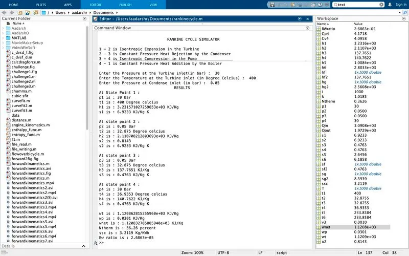
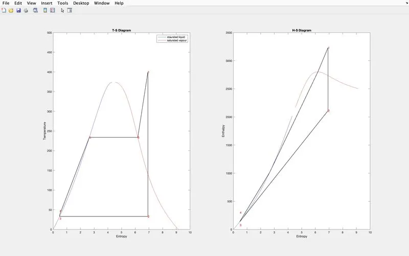
ERRORS OCCURED

Forgot to put END command after the loop which resulted in the popping of the following error message

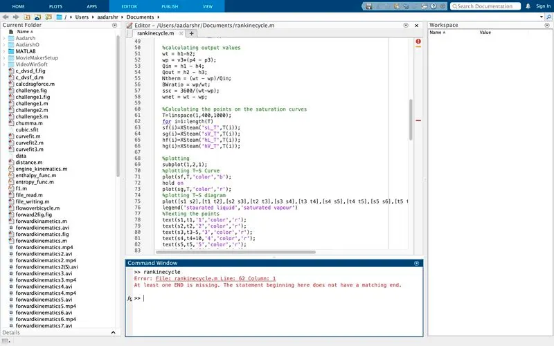
After putting the end command the program got executed

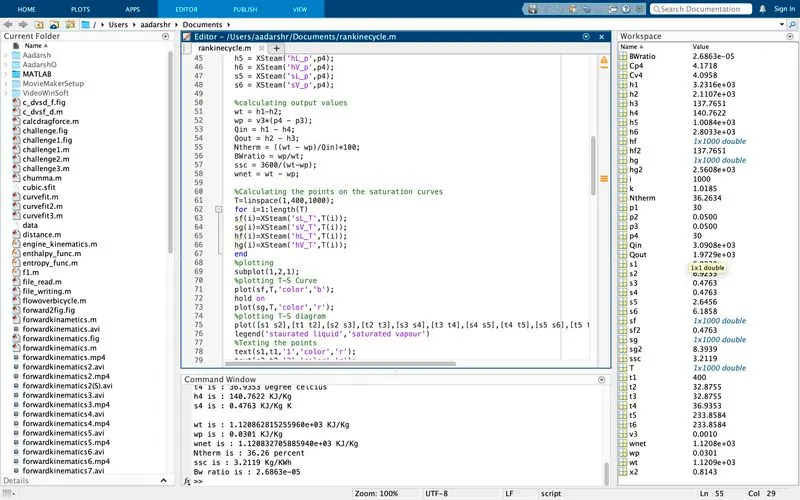
Without the end command the loop will not end and it will continue to run which makes it incomplete and the program will never get executed

RESULT

The program to simulate Rankine Cycle is completed and the follwing results are shown as output

At state point 1

p1 is : 30 Bar
t1 is : 400 Degree celcius
h1 is : 3.231571027259653e+03 KJ/Kg
s1 is : 6.9233 KJ/Kg K

At state point 2
p2 is : 0.05 Bar
t2 is : 32.875 Degree celcius
h2 is : 2.110708212003693e+03 KJ/Kg
x2 is : 0.8143
s2 is : 6.9233 KJ/Kg K

At state point 3
p3 is : 0.05 Bar
t3 is : 32.875 Degree celcius
h3 is : 137.7651 KJ/Kg
s3 is : 0.4763 KJ/Kg K

At state point 4
p4 is : 30 Bar
t4 is : 36.9353 Degree celcius
h4 is : 140.7622 KJ/Kg
s4 is : 0.4763 KJ/Kg K

wt is : 1.120862815255960e+03 KJ/Kg
wp is : 0.0301 KJ/Kg
wnet is : 1.120832705885940e+03 KJ/Kg
Ntherm is : 36.26 percent
ssc is : 3.2119 Kg/KWh
Bw ratio is : 2.6863e-05

Thermal efficiency of the cycle = 36.26%

Back Work Ratio =2.6863e-05

CONCLUSION

The program to create a Rankine Cycle Simulator is successfully carried out and the results are noted down as required.

Project 2 - Rankine cycle Simulator

Ship work like this
in your own course.

Talk to a career counsellor

Ship work like thisin your own course.

Talk to a career counsellor

Ship work like this
in your own course.