Week 3 - Solving second order ODEs
%program to solve an ODE which is the equation of motion of a pendulum
clear all
close all
clc
b = 0.05
g = 9.81
l = 1
m = 0.1

%initiall condition
theta_0 = [0;3]


%time points
t_span = linspace(0,20,200)


%solve ODE
[t, results] = ode45(@(t,theta)ode_func(t,theta,b,g,l,m),t_span,theta_0)

plot(t,results(:,1))

hold on
plot(t,results(:,2))
xlabel('plot')
ylabel('time')

%animation

disp = results(:,1)

ct = 1
for i =1:length(disp)

    x = 0
    y = 0
    x1 = l*sind(disp(i))
    y1 = -l*cosd(disp(i))
    plot([x x1],[y y1],'linewidth',3)
    hold on
    plot(x1,y1,'o','MarkerSize',20)
    plot([-3 3],[0 0],'linewidth',5)
    axis([-1 1 -1 1])
    hold off

    M(ct) = getframe(gcf)
    ct = ct+1
    end
%creating a videofile

movie(M);
videofile = VideoWriter('simplependulum','Uncompressed AVI');
open(videofile);
writeVideo(videofile,M);
close(videofile);
OUTPUT AND VIDEO
REPORT ON PROGRAM TO CREATE THE MOTION OF SIMPLE PENDULUM
AIM
A program to solve the ODE which represents the equation of the motion of a simple pendulum with damping
EQUATIONS USED
The equation of the motion of a simple pendulum with damping =
d^2(theta)/dt^2+(b/m)*d(theta)/dt+(g/l)*sin(theta)
d(theta1)/dt = theta2
d(theta2)/dt = -(b/m)*theta2-(g/l)*sin(theta1)
In the above equation theta1 which is equal to theta is the angular displacement and theta2 is the differential of theta1 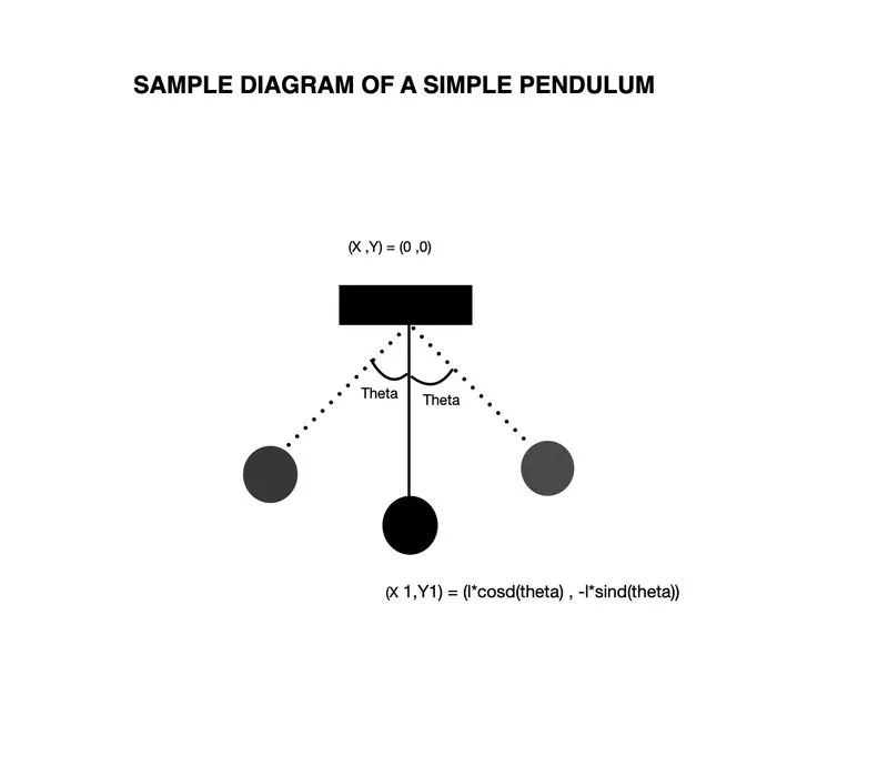
INPUTS
length of pendulum l = 1 m
damping coefficient b = 0.05
mass of the ball in kg = 0.1
gravity in m/s^2 = 9.81
initial conditions of displacement and velocity are 0 and 3 respectively
BODY OF CONTENT
The following is the step wise explanation of the program
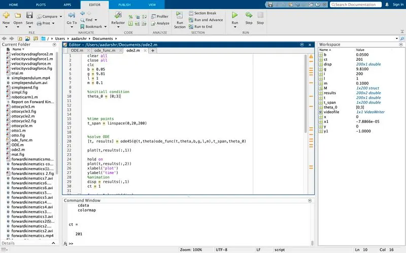
- The first step is the inputting of the initial conditions like theta_0 and t_span
%program to solve an ODE which is the equation of motion of a pendulum
clear all
close all
clc
b = 0.05
g = 9.81
l = 1
m = 0.1

%initiall condition
theta_0 = [0;3]


%time points
t_span = linspace(0,20,200)
The above program inputs the necessary values like b , g , l, m and the initial conditions like
theta_0 = [0;3] where for angular displacement theta the initial values of displacement and velocity are 0 and 3 respectively
similarly the time values are inputted using the linspace command which is as follows
t_span = linspace(0,20,200) , where the linspace command is used to give a time span from 0 to 2o seconds with 200 values in between
- The second step is to solve the ODE using ode45 command
- Before expalining the program a function called ode_func is defined as shown below
function [dtheta_dt] = ode_func(t,theta,b,g,l,m)
theta1 = theta(1)
theta2 = theta(2)
dtheta1_dt = theta2
dtheta2_dt = (-b/m)*theta2-(g/l)*(sin(theta1))
dtheta_dt = [dtheta1_dt;dtheta2_dt]
end
The function is stored in an array called [dtheta_dt] . The function is given the input values t , theta , b , g , l and m
Both the values of theta1 and theta2 are stored in a single variable 'theta' thus for storing those two values back into theta1 and theta2 we give the following command
theta1 = theta(1)
theta2 = theta(2)
Then we define our ODE i.e.
dtheta1_dt = theta2
%solve ODE
[t, results] = ode45(@(t,theta)ode_func(t,theta,b,g,l,m),t_span,theta_0)

plot(t,results(:,1))

hold on
plot(t,results(:,2))
xlabel('plot')
ylabel('time')
In the above command the time_span given as t and results are the variables into which the function ode45 is called. It is an in-built command used in MALAB
The main inputs are t and theta which are the variables of ODE system, then we define a function called ode_func with input parameters b,g,l and m, then we provide the time array i.e time span(t_span) and then the initial condition like and theta (theta_0) inside this command
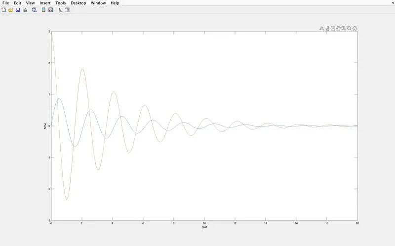
After that we plot a graph with time on x axis and results , which is a 200*2 matrix on y axis where in the plot there will be all the rows with only the first column i.e. the displacement column
using the plot command as shown below
plot(t,results(:,1))
similarly the graph between time and angular velocity is also plotted using the plot command as shown below
plot(t,results(:,2)) where (:,2) represents all the rows and the second column of the matrix.
we use a hold on command between the plot commands to avoid the overlapping of the two plots
The x axis is labelled as 'plot' and the y axis is labelled as 'time'
- The third stage is the animation creation step where we create an animation on the working of simple pendulum with the given values
disp = results(:,1)
ct = 1

for i =1:length(disp)

    x = 0
    y = 0
    x1 = l*sind(disp(i))
    y1 = -l*cosd(disp(i))
    plot([x x1],[y y1],'linewidth',3)
    hold on
    plot(x1,y1,'o','MarkerSize',20)
    plot([-3 3],[0 0],'linewidth',5)
    axis([-1 1 -1 1])
    hold off

    M(ct) = getframe(gcf)
    ct = ct+1
    end
In the above program at first we create a variablle called disp into which the results(:,1) is stored. The results(:,1) includes a matrix with 200 rows and 1 column. This is done to put the limits as length(disp) which is 200
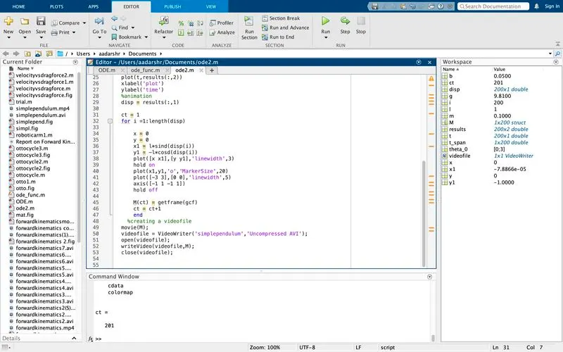
we keep the counter variable 'ct' set to 1 which counts upto a value of ct = 201 that is from 1 to 200
Next step is to use the for loop command for the motion of the pendulum from 1 to length(disp) which is 1 to 200.
Then we put the origin coordinates as (x,y) = (0,0)
the end coordinates are x1 = l*sind(disp(i))
y1 = -l*cosd(disp(i))
here the y1 coordinates are negative because the pendulum is hung from the origin to the negative y direction
disp(i) is the value from 1 to 200 when the program runs in each loop. i.e when i =1 disp(1), the first point of x1 , y1 is executed and the position of the pendulum changes along with it.
Then we plot the x , x1 and y, y1 using the plot command to generate a straight line between the origin and ( x1 , y1)
Then we plot the bob of the pendulum at (x1,y1) using the plot command and Marker command the command is as follows
plot(x1,y1,'o','Markersize',20)
here the 'o' is the shape of the bob and the size of the bob is determined using the command 'Markersize' with a valie of 20. A hold on command is used in between them to avoid overlapping of the two plots.
Then a command plot([-3 3] , [0 0],'linewidth',5) is used to create a plot which passes through the origin with (y , y1) = (0, 0) thus making it a horizontal line from -3 to 3 passing through the origin.
After that a fixed axis is given to the plot using the command axis([-1 1 -1 1])
Then we use hold off command to make the plot as required .
In the above program the individual frames are saved into an array i.e.'M' and then a command called 'getframe' is used to get the current figure window. Each frame is stored in that manner, which is later to be created as a movie. It is done using the command M(ct) = getframe(gcf)
After each loop the counter increments a value of 1 , which results in the execution of the next loop. At last the END command is used exit the loop.
- The last step is the creation of the movie using the create videofile command as shown below
movie(M);
videofile = VideoWriter('simplependulum','Uncompressed AVI');
open(videofile);
writeVideo(videofile,M);
close(videofile);- The movie is stored on to the variable M where the individual frames are saved.
- In the above command a movie is created and saved as 'simplependulum' using a videofile
- This videofile is opened using 'open(videofile)' command and is written into the array 'M' using the 'writevideo(videofile,M)' command
- Then the videofile is closed using 'close(videofile)' command
OUTPUT OF EACH PROGRAM
clear all
close all
clc
b = 0.05
g = 9.81
l = 1
m = 0.1

%initiall condition
theta_0 = [0;3]


%time points
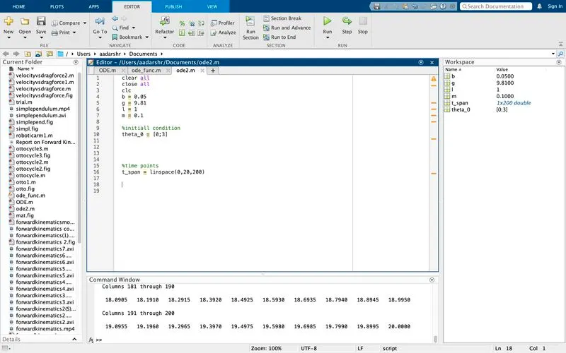
t_span = linspace(0,20,200)
OUTPUT
clear all
close all
clc
b = 0.05
g = 9.81
l = 1
m = 0.1

%initiall condition
theta_0 = [0;3]


%time points
t_span = linspace(0,20,200)


%solve ODE
[t, results] = ode45(@(t,theta)ode_func(t,theta,b,g,l,m),t_span,theta_0)

plot(t,results(:,1))

hold on
plot(t,results(:,2))
xlabel('plot')
ylabel('time')
OUTPUT
clear all
close all
clc
b = 0.05
g = 9.81
l = 1
m = 0.1

%initiall condition
theta_0 = [0;3]


%time points
t_span = linspace(0,20,200)


%solve ODE
[t, results] = ode45(@(t,theta)ode_func(t,theta,b,g,l,m),t_span,theta_0)

plot(t,results(:,1))

hold on
plot(t,results(:,2))
xlabel('plot')
ylabel('time')
%animation
disp = results(:,1)
ct = 1

for i =1:length(disp)

    x = 0
    y = 0
    x1 = l*sind(disp(i))
    y1 = -l*cosd(disp(i))
    plot([x x1],[y y1],'linewidth',3)
    hold on
    plot(x1,y1,'o','MarkerSize',20)
    plot([-3 3],[0 0],'linewidth',5)
    axis([-1 1 -1 1])
    hold off

    M(ct) = getframe(gcf)
    ct = ct+1
    end
  %creating a videofile
movie(M);
videofile = VideoWriter('simplependulum','Uncompressed AVI');
open(videofile);
writeVideo(videofile,M);
close(videofile);
OUTPUT
. .
For t_span(0,20,100)
OUTPUT
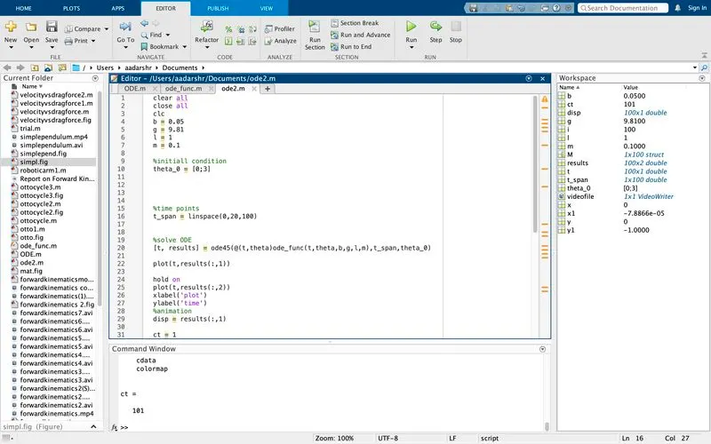
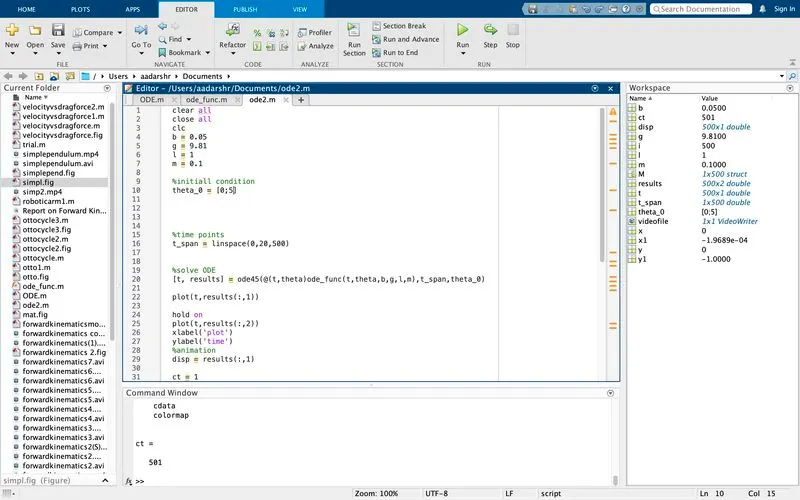
For theta_0 = [0;5] , t_span = (0,20,500)
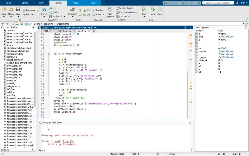
ERRORS OCCURED
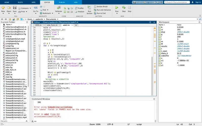
Forgot to input counter 'ct' =1. The counter variable is necessary to count the frames without it the program will not get executed.
After putting 'ct =1' program got executed
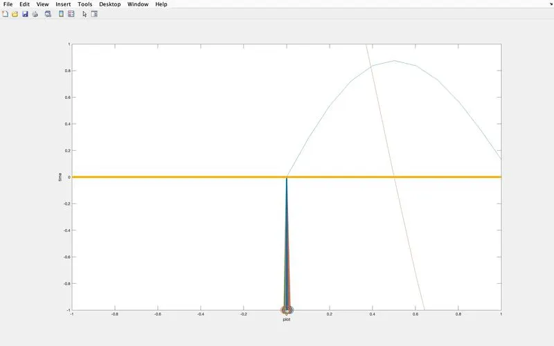
Forgot to use hold off command
 .
. 
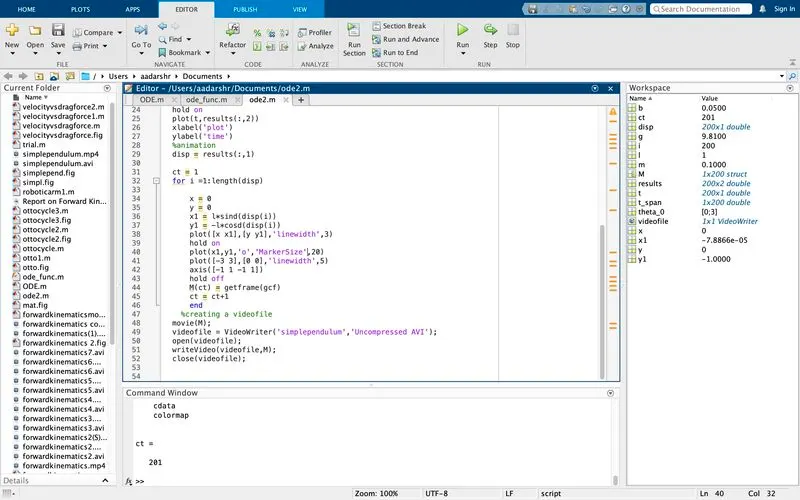
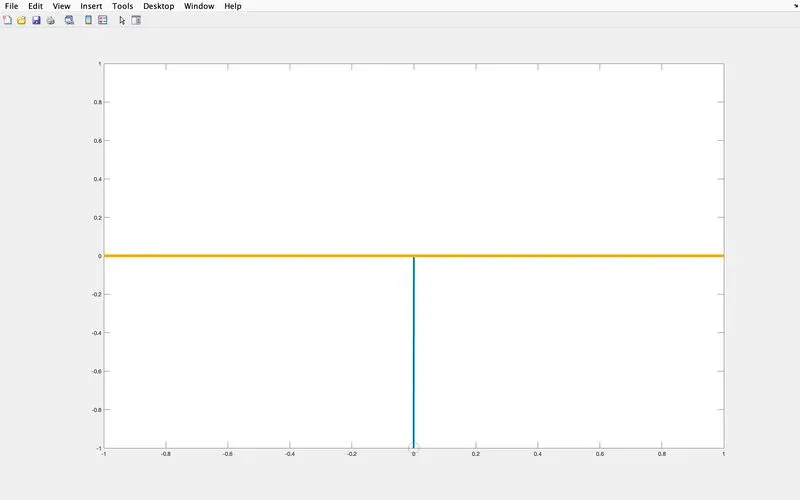
After putting hold off command
.
RESULT
The final result is an array of 200 rows and 1 column
The youtube link is : https://youtu.be/alDnsiVvG8U
CONCLUSION
The program to create a ODE which is the equation of a simple pendulum with damping is successfully executed and the final values of angular displacement and angular velocity are noted.
The video of working of the simple pendulum using the given values is also created and uploaded on youtube.
.