Week 4.1 - Genetic Algorithm
AIM
To write a program to optimise stalagmite function and find global maxima of the function
EQUATIONS USED
stalg = -stalg1
- Initialisation : It is the process of initialising the size of the population by deciding how much population is to be assumed so that the algorithm can be computed. If more population is assumed more accurate will be the results
- Selection : In this process parents are selected , the selection process is carried out according to Darwin's theory that is " survival of the fittest" , which implies that the fittest of all will be selected and proceeded forward for creating next generation. In this process the best parents are selected and new best generations
- Crossover : The process of interchanging of genes of two parents is known as crossover
- Mutation : Mutation is carried out to maintain the genetic diversity from one generation to next. if it is not done the further generations will be similar andd there will be no diversity.
GA is mainly used in optimisation problems but it is also ued in the field of Economics, Neural networks, Image processing etc.
Syntax for ga
- x = ga(fun,nvars) finds a local unconstrained minimum, x, to the objective function, (fun, nvars) is the dimension (number of design variables) of fun.
-
x = ga(fun,nvars,A,b,Aeq,beq,lb,ub) defines a set of lower and upper bounds on the design variables, x, so that a solution is found in the range lb ≤ x ≤ ub. (Set Aeq=[] and beq=[] if no linear equalities exist.) lb and ub are the lower and upper bounds
-
x = ga(fun,nvars,A,b,Aeq,beq,lb,ub,nonlcon,options) minimizes with the default optimization parameters replaced by values in options. Set nonlcon=[] if no nonlinear constraints exist. Create options using optimoptions.
-
x = ga(fun,nvars,A,b,Aeq,beq,lb,ub,nonlcon,intcon,options) requires that the variables listed in intcon take integer values. If intcon is 0 then we give intcon = []
BODY OF CONTENT
clear all
close all
clc
%defining our search space
x = linspace(0,0.6,150);
y = linspace(0,0.6,150);
num_cases = 50
%conversion of x and y into 2D
[xx yy] = meshgrid(x,y)

%calling function using for loop

for i = 1:length(xx)
    for j = 1:length(yy)
        input_vector(1) = xx(i,j);
        input_vector(2) = yy(i,j);
        f(i,j) = stalagmite(input_vector);
    end
end
In the above program we first take two random variables x and y and input the values ranging from 0 to 0.6 using linspace command and also we provide 150 values in between them.
Then we input the number of times the GA should run using the variable num_cases = 50
The next step is to convert x and y into 2D using meshgrid command. After that we call the function stalagmite using for loop
The stalagmite function is as follows
function [stalg] = stalagmite(input_vector)
f1_x = (sin((5.1*pi.*input_vector(1))+0.5)).^6
f1_y = (sin((5.1*pi.*input_vector(2))+0.5)).^6
f2_x = exp(-4 *log(2).*((input_vector(1)-0.0667)^2)/0.64)
f2_y = exp(-4 *log(2).*((input_vector(2)-0.0667)^2)/0.64)
stalg1 = (f1_x*f2_x*f1_y*f2_y)
stalg = -stalg1
end
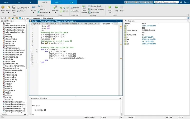
In the above function stalag is defined as stalagmite with input _vector as the input values. The input vector consists of xx and yy values .
Then we define the equation which is the objective function to carry out the GA. For that we define f1_x, f1_y, f2_x , f2_y as shown above. It is done to evaluate the individual functions of the main function 'stalg'. Here function stalg is given the name stalg1 so that the function stalg becomes -(stalg1) which is defined in the next step. This is done to calculate the global minima which is later converted into Global maxima later in the program. Then we end the function
In the for loop we give the limits of i loop from 1 to length(xx) and the j loop from 1 to length(yy) ,where the length((xx) and (yy)) are 150 each.
Then the values in xx and yy are stored into the variable named input_vector(1) and input_vector(2) respectively i.e
tic
%Study 1 - statistical behaviour
for i = 1:num_cases
    [inputs,fopt(i)] = ga(@stalagmite,2)
    xopt(i) = inputs(1)
    yopt(i) = inputs(2)
end
study1_time = toc
%plotting
figure(1)
subplot(2,1,1)
hold on
surf(x,y,-f)
shading interp
plot3(xopt,yopt,-fopt,'marker','o','MarkerSize',5,'MarkerFaceColor','r')
title('unbounded inputs')
subplot(2,1,2)
plot(-fopt)
xlabel('Iterations')
ylabel('Function maximum')
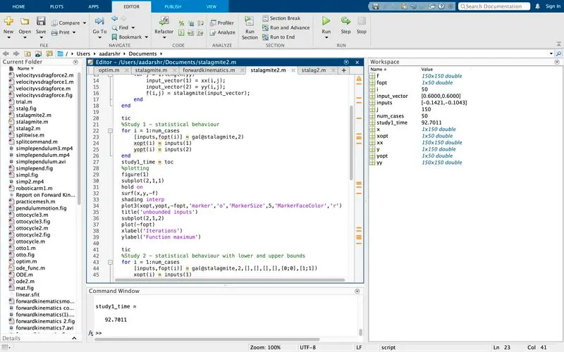
In the above program first we give a tic command followed by study1_time = toc command which is used to calculate the time taken to compute the optimised values for the GA
Here we use a for loop i which varies from 1 to num_cases (which is 50) and we call the function stalagmite into an array which consists of inputs and optimised f values which is calculated for each loop. Where the command ga(@stalagmite,2) is the ga function command which takes the function stalagmite and the number of variables (i.e. 2) as input and calculate the minimum value of the function.
Then we input the values of x and y which is stored as input(1) and input(2) into xopt and yopt respectively. Where xopt and yopt are the optimum values of x and y.
Now we plot the values of x , y, f on a plot using subplot command. Subplot command is used to plot 2 or more plots in a single plot window. Where in the above program the command is given as follows subplot(2,1,1) it plots a matrix with 2 rows and 1 column with marking on the first row.
Then surf command is used to create the surface obtained with respect to the plotting. Hold on command is used in between them to avoid overlapping of the plots.
We then give shading interp command so that the lines appeared after executing surf command disappears inorder to get a more clear and clean plot.
Then we plot the 3D plot with the xopt, yopt and fopt where fopt is the optimised value of f corresponding to xopt and yopt which is the required value in the z direction.The command is shown below
Here the fopt is plotted as -fopt so that the plot shows the global maxima( f) which is required.
It is given a title as 'unbounded inputs' and then another subplot is created to plot the values of function maximum using the subplot command
We then plot the optimised global minima fopt as -fopt so that the plot generated is in the positive axis and the value of global maxima is created.
Then we label the x axis as 'iterations' and y axis as 'Function maximum'
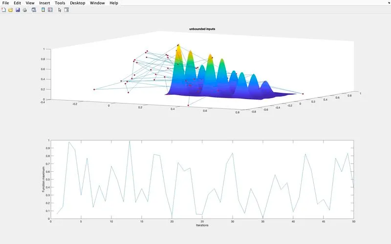
In the above program the output obtained shows different global maximas due to the inputting of random values which is incorrect as shown below
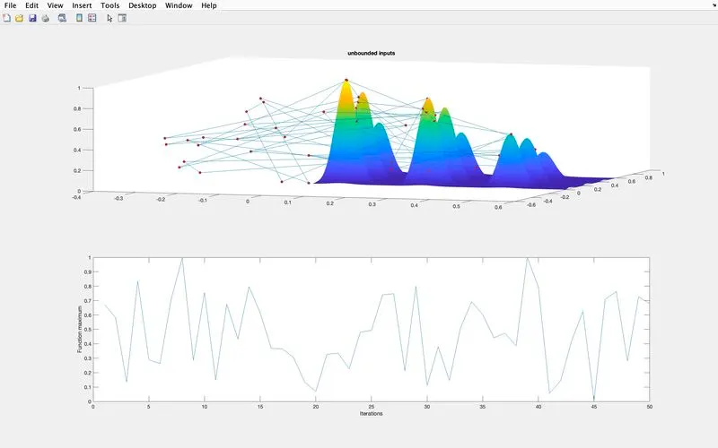
In the above plot there are more than one function maximums which makes it difficult to find which is the most suited one, thus to make it converge into a more convincing one we use boundary commands in the ga function which is given in the following manner
x = ga(fun,nvars,A,b,Aeq,beq,lb,ub) which defines a set of lower and upper bounds on the design variables, x, so that a solution is found in the range lb ≤ x ≤ ub, lb and ub are the lower and upper bounds
This function is used in place of x = ga(fun,nvars) inorder to compute a more optimised function maximum value. This is the second step of the program which is labelled as the statistical behaviour with upper and lower bounds
tic
%Study 2 - statistical behaviour with lower and upper bounds
for i = 1:num_cases
    [inputs,fopt(i)] = ga(@stalagmite,2,[],[],[],[],[0;0],[1;1])
    xopt(i) = inputs(1)
    yopt(i) = inputs(2)
end

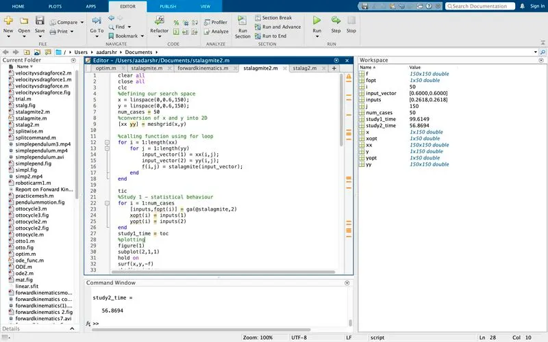
study2_time = toc
figure(2)
subplot(2,1,1)
hold on
surf(x,y,-f)
shading interp
plot3(xopt,yopt,-fopt,'marker','o','MarkerSize',5,'MarkerFaceColor','r')
title('unbounded inputs')
subplot(2,1,2)
plot(-fopt)
xlabel('Iterations')
ylabel('Function maximum')
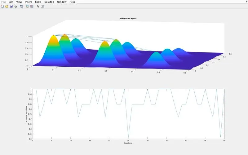
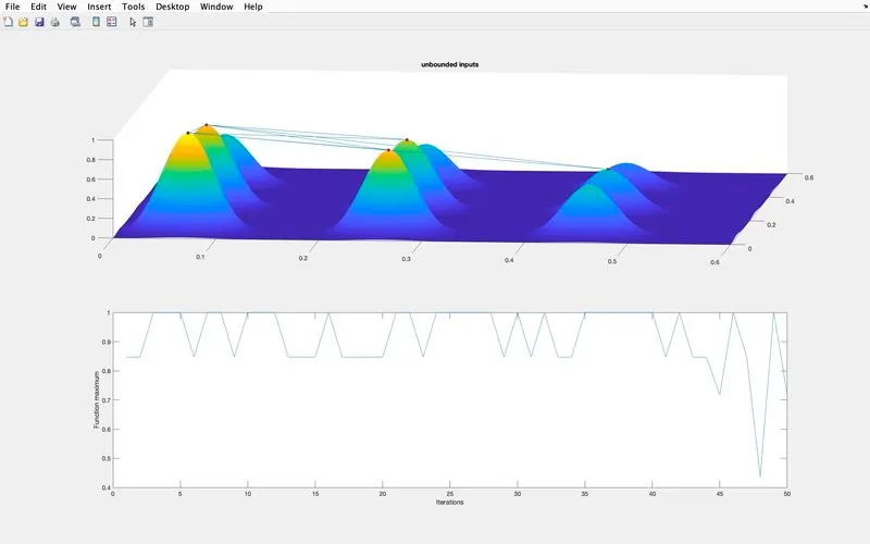
In the above program the only difference is in the function definition where lower and upper bounds are given , so that the output generated will have a value between 0 and 1 , with 0 as the global minimum and 1 as global maxima. The function is as follows
tic
%Study 3 - increase the Ga iterations
options = optimoptions('ga')
options = optimoptions('ga','PopulationSize',200)
for i =1:num_cases
[inputs,fopt(i)] = ga(@stalagmite,2,[],[],[],[],[0;0],[1;1],[],[],options)
    xopt(i) = inputs(1)
    yopt(i) = inputs(2)
end
study3_time = toc
figure(3)
subplot(2,1,1)
hold on
surf(x,y,-f)
shading interp
plot3(xopt,yopt,-fopt,'marker','o','MarkerSize',5,'MarkerFaceColor','r')
title('bounded inputs with increase in iterations')
subplot(2,1,2)
plot(-fopt)
xlabel('Iterations')
ylabel('Function maximum')
In the above program we increase the ga iterations using optimoptions command , the command helps in changing the parameters as per the requirement
options = optimoptions('ga') returns a set of default options for the ga solver.
options = optimoptions('ga','PopulationSize,200) returns options with specified parameters set using one or more name-value pair arguments. Here we give 200 as the population size inorder to converge the global maxima into a single value.
Then function definition with options as input is carried out.
x = ga(fun,nvars,A,b,Aeq,beq,lb,ub,nonlcon,intcon,options) requires that the variables listed in intcon take integer values. If intcon is 0 then we give intcon = [] where nonlcon is the non linear constraints and intcon is the integer constraints . Since there are no nonlinear or integer constraints present we give empty brackets in place of that. The function definition for the program above is carried out inside the for loop. The process is repeated until an optimised result is found out.
Here we use a for loop i which varies from 1 to num_cases (which is 50) and we call the function stalagmite into an array which consists of inputs and optimised f values which is calculated for each loop. Where the command ga(@stalagmite,2,[],[],[],[],[0;0],[1;1],[],[],options) is the ga function command which takes the function stalagmite and the number of variables (i.e. 2) as input and calculate the minimum value of the function.
Then we input the values of x and y which is stored as input(1) and input(2) into xopt and yopt respectively. Where xopt and yopt are the optimum values of x and y.
Now we plot the values of x , y, f on a plot using subplot command. Subplot command is used to plot 2 or more plots in a single plot window. Where in the above program the command is given as follows subplot(2,1,1) it plots a matrix with 2 rows and 1 column with marking on the first row.
Then surf command is used to create the surface obtained with respect to the plotting. Hold on command is used in between them to avoid overlapping of the plots.
We then give shading interp command so that the lines appeared after executing surf command disappears inorder to get a more clear and clean plot.
Then we plot the 3D plot with the xopt, yopt and fopt where fopt is the optimised value of f corresponding to xopt and yopt which is the required value in the z direction.The command is shown below
Here the fopt is plotted as -fopt so that the plot shows the global maxima( f) which is required.
It is given a title as 'unbounded inputs' and then another subplot is created to plot the values of function maximum using the subplot command
We then plot the optimised global minima fopt as -fopt so that the plot generated is in the positive axis and the value of global maxima is created.
Then we label the x axis as 'iterations' and y axis as 'Function maximum'
OUTPUTS OF PROGRAMS
Basic program
clear all
close all
clc
%defining our search space
x = linspace(0,0.6,150);
y = linspace(0,0.6,150);

[xx yy] = meshgrid(x,y)

for i = 1:length(xx)
    for j = 1:length(yy)
        input_vector(1) = xx(i,j);
        input_vector(2) = yy(i,j);
        f(i,j) = stalagmite(input_vector);
    end
end
surf(xx,yy,f)
shading interp
xlabel('x axis')
ylabel('y axis')
[inputs,fval] = ga(@stalagmite,2)
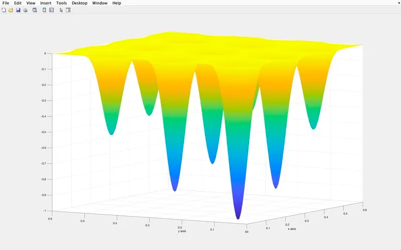
OUTPUT
clear all
close all
clc
%defining our search space
x = linspace(0,0.6,150);
y = linspace(0,0.6,150);
num_cases = 50
%conversion of x and y into 2D
[xx yy] = meshgrid(x,y)

%calling function using for loop
for i = 1:length(xx)
    for j = 1:length(yy)
        input_vector(1) = xx(i,j);
        input_vector(2) = yy(i,j);
        f(i,j) = stalagmite(input_vector);
    end
end
OUTPUT
For study 1 - Statistical behaviour
clear all
close all
clc
%defining our search space
x = linspace(0,0.6,150);
y = linspace(0,0.6,150);
num_cases = 50
%conversion of x and y into 2D
[xx yy] = meshgrid(x,y)

%calling function using for loop
for i = 1:length(xx)
    for j = 1:length(yy)
        input_vector(1) = xx(i,j);
        input_vector(2) = yy(i,j);
        f(i,j) = stalagmite(input_vector);
    end
end

tic
%Study 1 - statistical behaviour
for i = 1:num_cases
    [inputs,fopt(i)] = ga(@stalagmite,2)
    xopt(i) = inputs(1)
    yopt(i) = inputs(2)
end
study1_time = toc
%plotting
figure(1)
subplot(2,1,1)
hold on
surf(x,y,-f)
shading interp
plot3(xopt,yopt,-fopt,'marker','o','MarkerSize',5,'MarkerFaceColor','r')
title('unbounded inputs')
subplot(2,1,2)
plot(-fopt)
xlabel('Iterations')
ylabel('Function maximum')
OUTPUT AND PLOT
For study 2 - Statistical behaviour using lower and upper bounds
clear all
close all
clc
%defining our search space
x = linspace(0,0.6,150);
y = linspace(0,0.6,150);
num_cases = 50
%conversion of x and y into 2D
[xx yy] = meshgrid(x,y)

%calling function using for loop
for i = 1:length(xx)
    for j = 1:length(yy)
        input_vector(1) = xx(i,j);
        input_vector(2) = yy(i,j);
        f(i,j) = stalagmite(input_vector);
    end
end

tic
%Study 1 - statistical behaviour
for i = 1:num_cases
    [inputs,fopt(i)] = ga(@stalagmite,2)
    xopt(i) = inputs(1)
    yopt(i) = inputs(2)
end
study1_time = toc
%plotting
figure(1)
subplot(2,1,1)
hold on
surf(x,y,-f)
shading interp
plot3(xopt,yopt,-fopt,'marker','o','MarkerSize',5,'MarkerFaceColor','r')
title('unbounded inputs')
subplot(2,1,2)
plot(-fopt)
xlabel('Iterations')
ylabel('Function maximum')

tic
%Study 2 - statistical behaviour with lower and upper bounds
for i = 1:num_cases
    [inputs,fopt(i)] = ga(@stalagmite,2,[],[],[],[],[0;0],[1;1])
    xopt(i) = inputs(1)
    yopt(i) = inputs(2)
end

study2_time = toc
figure(2)
subplot(2,1,1)
hold on
surf(x,y,-f)
shading interp
plot3(xopt,yopt,-fopt,'marker','o','MarkerSize',5,'MarkerFaceColor','r')
title('unbounded inputs')
subplot(2,1,2)
plot(-fopt)
xlabel('Iterations')
ylabel('Function maximum')
OUTPUT AND PLOT
For study 3 - increasing GA iterations
clear all
close all
clc
%defining our search space
x = linspace(0,0.6,150);
y = linspace(0,0.6,150);
num_cases = 50
%conversion of x and y into 2D
[xx yy] = meshgrid(x,y)

%calling function using for loop
for i = 1:length(xx)
    for j = 1:length(yy)
        input_vector(1) = xx(i,j);
        input_vector(2) = yy(i,j);
        f(i,j) = stalagmite(input_vector);
    end
end

tic
%Study 1 - statistical behaviour
for i = 1:num_cases
    [inputs,fopt(i)] = ga(@stalagmite,2)
    xopt(i) = inputs(1)
    yopt(i) = inputs(2)
end
study1_time = toc
%plotting
figure(1)
subplot(2,1,1)
hold on
surf(x,y,-f)
shading interp
plot3(xopt,yopt,-fopt,'marker','o','MarkerSize',5,'MarkerFaceColor','r')
title('unbounded inputs')
subplot(2,1,2)
plot(-fopt)
xlabel('Iterations')
ylabel('Function maximum')

tic
%Study 2 - statistical behaviour with lower and upper bounds
for i = 1:num_cases
    [inputs,fopt(i)] = ga(@stalagmite,2,[],[],[],[],[0;0],[1;1])
    xopt(i) = inputs(1)
    yopt(i) = inputs(2)
end

study2_time = toc
figure(2)
subplot(2,1,1)
hold on
surf(x,y,-f)
shading interp
plot3(xopt,yopt,-fopt,'marker','o','MarkerSize',5,'MarkerFaceColor','r')
title('unbounded inputs')
subplot(2,1,2)
plot(-fopt)
xlabel('Iterations')
ylabel('Function maximum')

tic
%Study 3 - increase the Ga iterations
options = optimoptions('ga')
options = optimoptions('ga','PopulationSize',200)
for i =1:num_cases
[inputs,fopt(i)] = ga(@stalagmite,2,[],[],[],[],[0;0],[1;1],[],[],options)
    xopt(i) = inputs(1)
    yopt(i) = inputs(2)
end
study3_time = toc
figure(3)
subplot(2,1,1)
hold on
surf(x,y,-f)
shading interp
plot3(xopt,yopt,-fopt,'marker','o','MarkerSize',5,'MarkerFaceColor','r')
title('bounded inputs with increase in iterations')
subplot(2,1,2)
plot(-fopt)
xlabel('Iterations')
ylabel('Function maximum')
OUTPUT AND PLOT
ERRORS OCCURRED
Forgot to put END command for the j loop which rresulted in the popping of the following error message
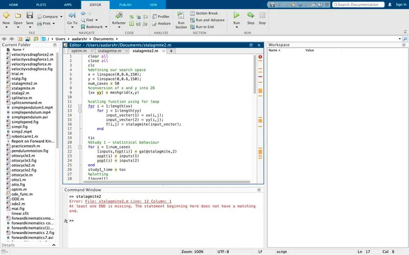
The END command is necessary because it helps the for loop to understand when to stop the loop for the execution of the program, without it the program will not get executed
After putting END command the program got executed
RESULT
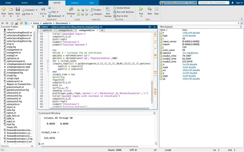
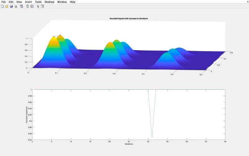
The global maxima fopt = 1 and the study took 223 seconds to complete the execution. The input_vector =[ 0.0668 0.0668]
Thus it shows that increasing the population size helps in getting more optimised result
CONCLUSION
A program to calculate the global maxima using otimisation technique in stalagmite function is successfully carried out and the results are noted.
REFERENCE
MATHWORKS, https://www.tutorialspoint.com/genetic_algorithms/genetic_algorithms_introduction.htm , google, wikipedia