Week 8 - Simulation of a backward facing step in OpenFOAM

Aim:

To simulate an incompressible-laminar-viscous flow through the backward facing step geometry. We should perform a transient simulation. The solver can be chosen based on the described physics of the flow. We need to explain the entire simulation procedure (how you set up the case). You should also provide explanations to every change you make inside the reference case files obtained from OpenFOAM tutorials. We can choose the inlet velocity such that the flow is laminar.

Objective:

We have to find out below the given values

Case 1 - Simulate the flow without using any grading factor (i.e., GF = 1)

Case 2 - Simulate the flow with grading factor of 0.2. The cells should be finer near the walls (including the step wall).

Mesh specification

1. Number of cells along the x direction (longer dimension) = 200
2. Number of cells along the longer y direction = 20;

Desired output

• Measure the velocity profile at 0.085 m from the inlet of the geometry for both case studies and compare. You can use the plot over line tool for this.
• Explain why Grading/Growth factor is essential for meshing.

Geometry:

The Block mesh dict file is used for creating geometry, generating mesh and defining boundary condition.

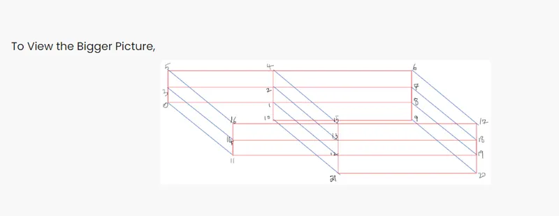
The following procedures needed to be followed in creating geometry in Blockmesh.

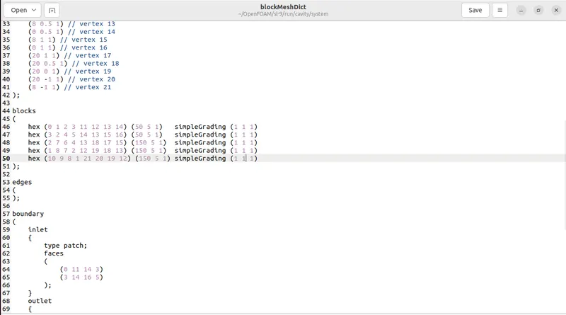
The whole part is created by using a combination of 5 blocks.

At first, vertices should be defined for each block ie. 1,2.

After that we have to creating blocks, meshing is done by using hex

below this represent the seperate the blocks and give the block numbers

Explanation:

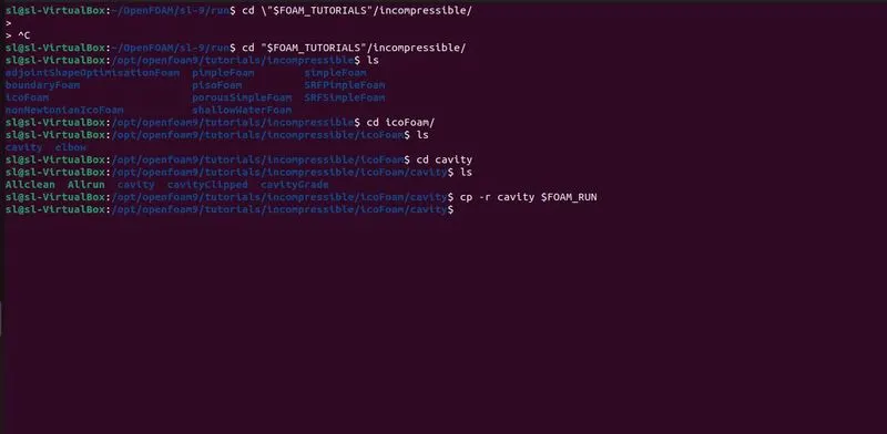
• This is a challenge of incompressible laminar viscous flow, we use cavity folder in tutorial.
• We have to create a copy of cavity folder from tutorial in the $FOAM_RUN folder with a name cavity and cavity.
• Then open cavity folder which has 3 folders 0, constant and system.
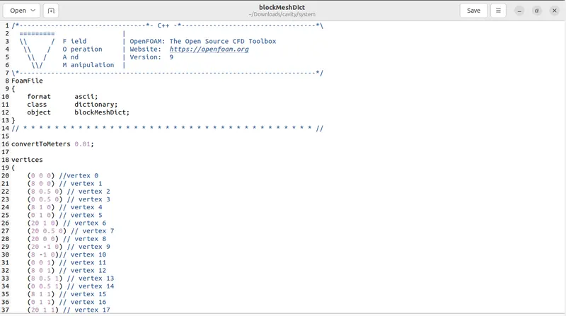
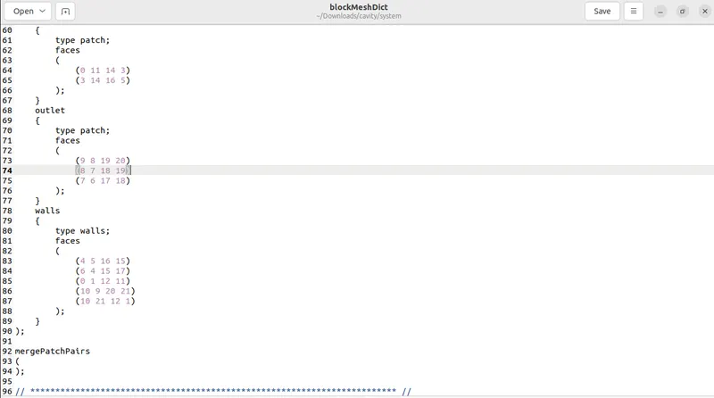
• The blockmeshdict text File then specify the vertices as per the given dimensions of the backward facing step (in Geometry) specify the hex block mesh with given mesh specification with grading factor of 1 1 1 in x y and z directions respectively.
• We have to specify the inlet and outlet with type patch, front and back walls with type empty and noslipwall with type wall. save the blockMeshdict text file.
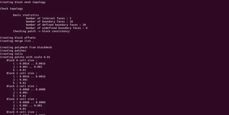
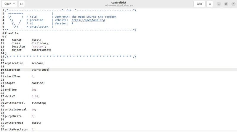
• Type blockMesh in the windows terminal to create meshing. once you create meshing, open controldict text file and specify the start time, end time, time step, dt and write interval.
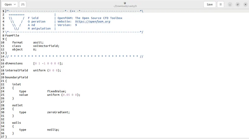
• Go to folder 0 in the cavity file. open U text file and specify the velocity at the inlet as 1m/s, outlet as zero gradient, front and back as empty and noslipwalls as zero gradient and save.
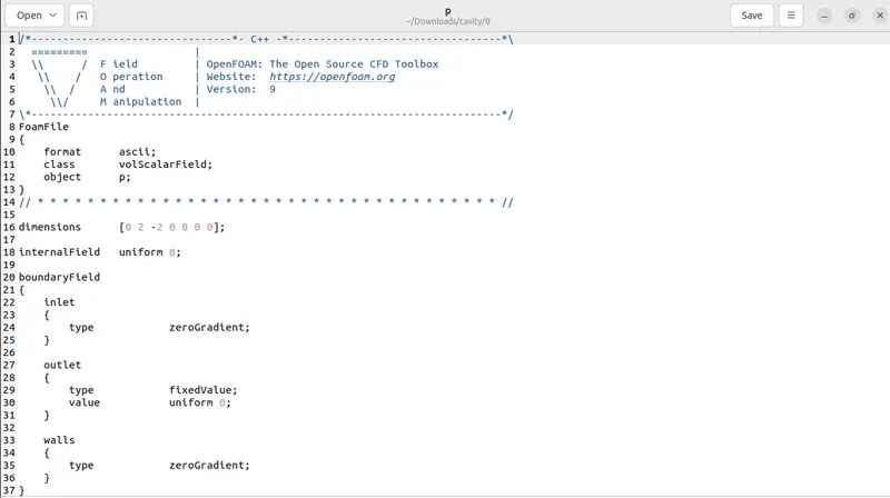
• open p text file and specify the pressure at the inlet as zero gradient, outlet as fixed and uniform 0, front and back as empty and noslipwalls as zero gradient and save.
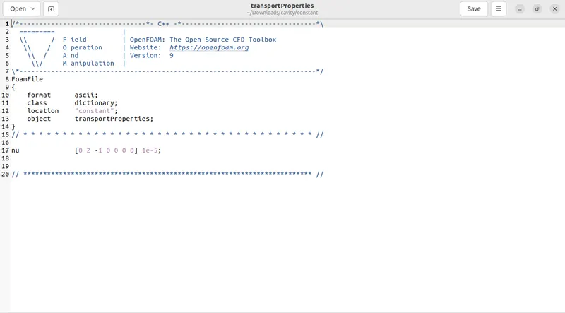
• After that we have to specifying the velocity and pressure as boundary conditions open folder constant and open text file transport properties specify the value of kinematic viscosity then save.
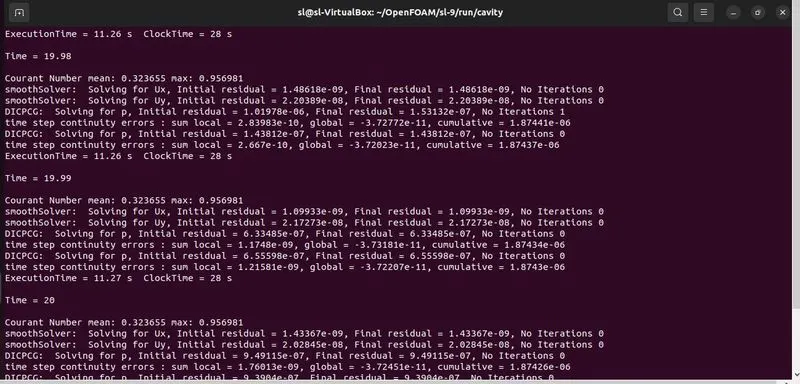
• Then come back to main run folder and run icofoam application for simulation. Finally, the solution will converge and depending on the time step and dt.
• We have to Cross checked by the courant number which should be less than 1.
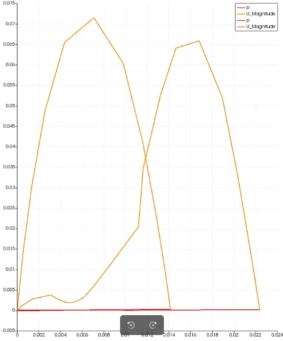
• Plot a graph to find the variation of velocity at a distance of 0.085m. same procedure is repeated for cavity with a gradient factor of 0.2 and plot the variation of velocity at a distance of 0.085m.

blockMeshDict: (for Gradient factor of 0.2)

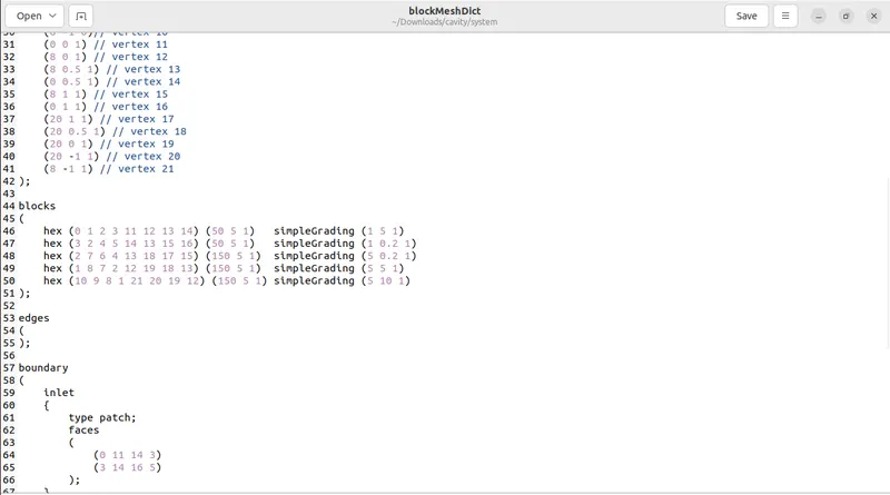
blockMeshDict: (for Gradient factor of 1)

Blockmesh output image:

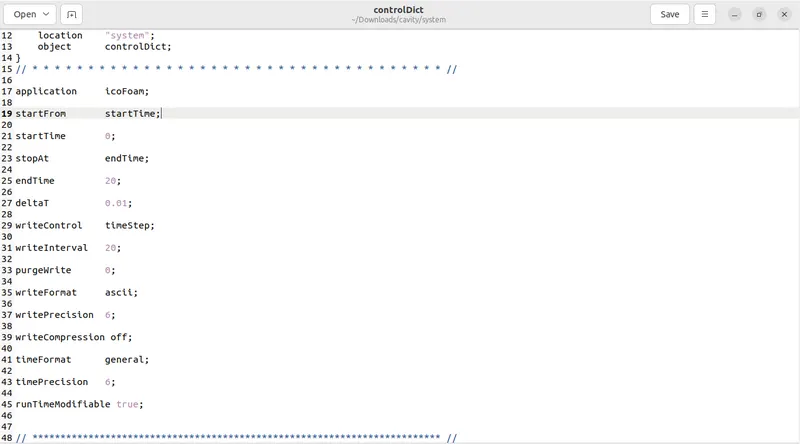
Controldict image:

The Controldict time steps can be controlled in the controldict file. In this simulation start and end time is provided as 0 and 20. deltaT is assumed to be 0.01.

Transport properties image:

Pressure image:

Initial condition: The initial condition for velocity and pressure can be provided in the p and U file located in the 0 folder.

Velocity image:

Initial condition: The initial condition for velocity and pressure can be provided in the p and U file located in the 0 folder.

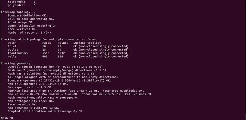
Checkmesh image:

icoFoam image:

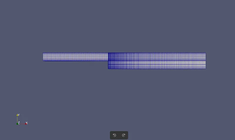
GF = 0.2

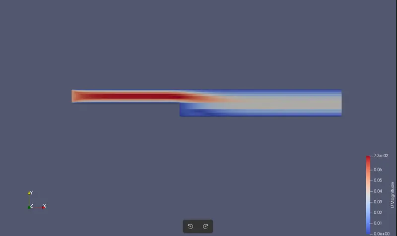
velocity distribution in backward facing step:

plot of variation of velocity with GF = 0.2 at the walls.( at a distance 0.085m )

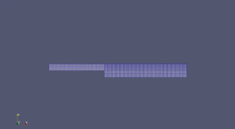
Mesh image GF = 1

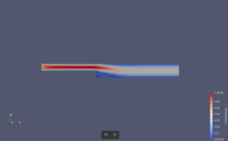
velocity distribution in backward facing step:

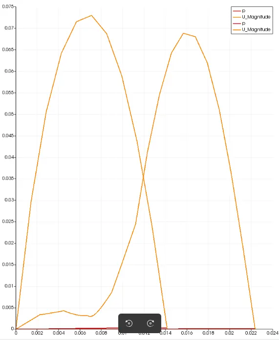
Plot of variation of velocity: at a distance 0.085m
with GF =1

CONCLUSION:

Finally, we have to conclude from the graph it’s clear that as with the increase in the fine mesh with GF =0.2 the curve is bit smoother to capture the velocity at the specific point whereas for the coarse mesh with GF = 1 the curve is bit short at the peak and hence for capturing more accurate results at the specific point the mesh can be made finer instead of coarse mesh the accuracy of results is more. However the computation time increases with finer mesh.