Week 8 - Simulation of a backward facing step in OpenFOAM

• AIM:

The main aim of the challenge is to simulate an incompressible-laminar-viscous flow through the backward facing step geometry using openFoam.

• OBJECTIVE:

Backward Facing Step (BFS) is widely known for its application in the studies on turbulence in internal flows. The flow separation is caused due to the sudden changes in the geometry. This creates a zone of re-circulation and a point of flow reattachment.

PROBLEM STATEMENT:

Simulate an incompressible-laminar-viscous flow through the backward facing step geometry and perform 2 case studies as described below and compare the results

CASE 1: Simulate the flow without using any grading factor (GF=1)

CASE 2: Simulate the flow with grading factor of 0.2.The cells should be finer near the walls

MESH SPECIFICATION:

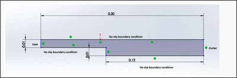
1. Number of cells along the x direction = 200
2. Number of cells along the y direction = 20

BOUNDARY SPECIFICATION:

The domain specification are provided in the following figure.

STEPS:

• Open openFoam tutorials and find the solver which solves the physics of the given problem.
• Next is to copy required file in solver and paste it in openFoam run folder.
• Find the blockMeshdict file and alter according to the given geometry.
• Find controldict file to edit start and end time of the simulation.
• In initial folder '0' initialize the pressure and velocity according to the given domain.
• Use blockMesh command to generate the mesh on the geometry.
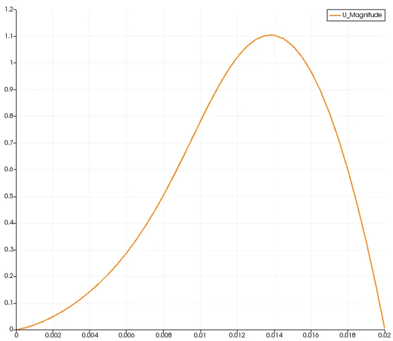
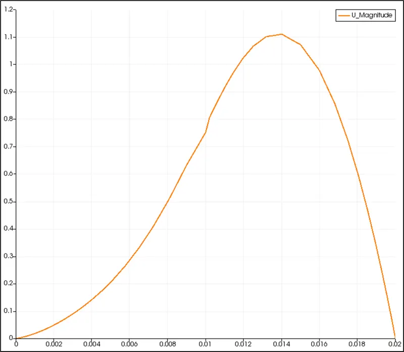
• Open simulation file in paraview and plot the velocity profile at point 0.085m from the inlet.
• Repeat the above procedure for the case 2 and check the difference in the results.

CASE 1:

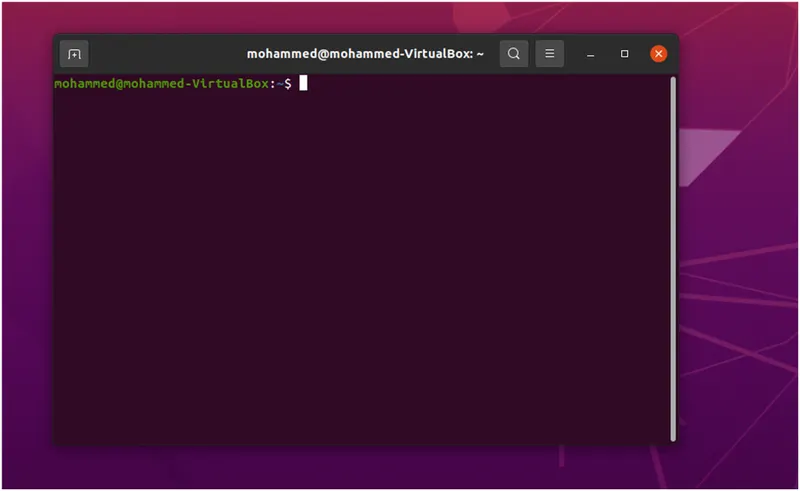
In order to start simulation process first start the terminal in LINUX operating system using ctrl+alt+T button

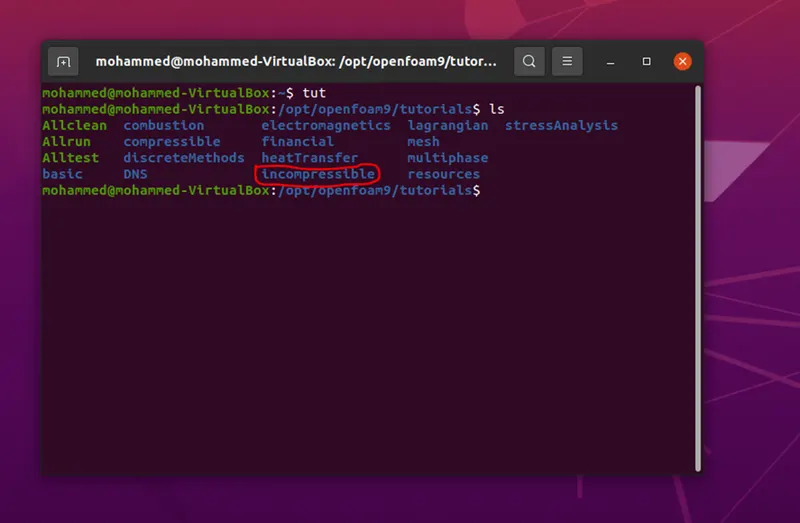
Now,we are going to solve our problem using tutorials present in openFoam,therefore type 'tut' in terminal to navigate to the tutorial directory of openFoam and type 'ls' to get the list of tutorials present in that directory.We are going to solve for incompressible flow simulation so select the suitable directory.

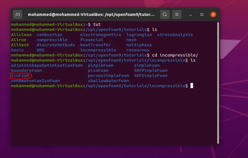
icoFoam is the solver in openFoam which is use as transient solver for incompressible-laminar flow of Newtonian fluids.Therfore we select icoFoam and we find list of folders in that directory and we are going to select the cavity folder for this problem statement.

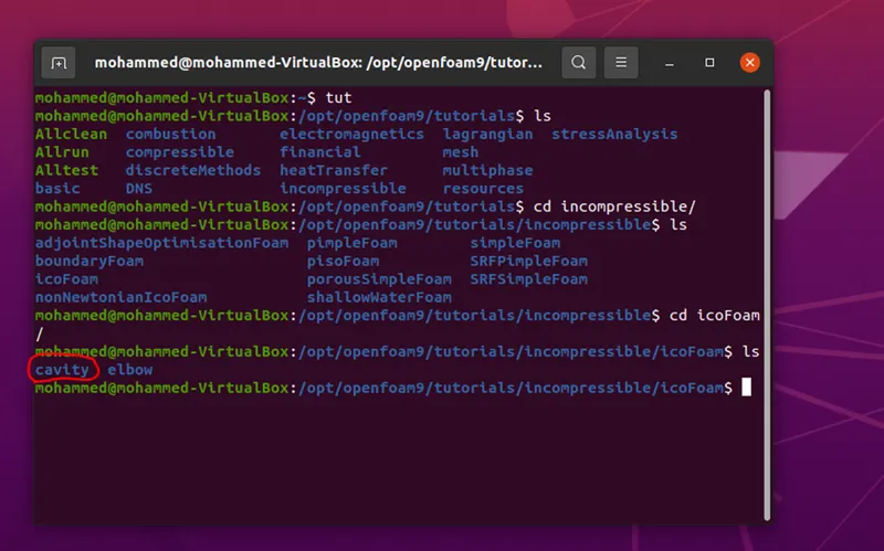
We are going to copy cavity folder to the run folder and simulate the same in the run folder.

In system directory we have blockMeshDict file which we have to alter to match to given problem geometry.

When we open this file we are going to see header information in the form of comment which is not executable

Then,we will observe the file which identify by the openFoam reads to understand in this case it is 'blockMeshDict'

MESH GENERATION WITHOUT GRADING FACTOR:

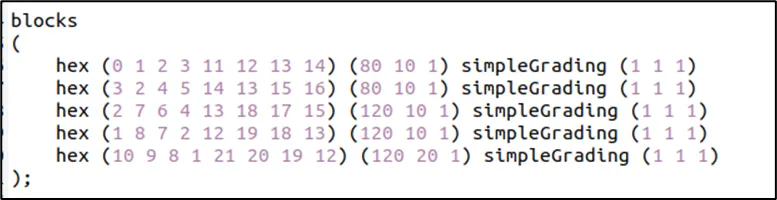
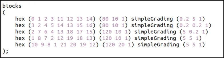
In the same file we can see the hex and that is the line where we specify the faces of the blocks and also number of cells in X,Y and Z direction.

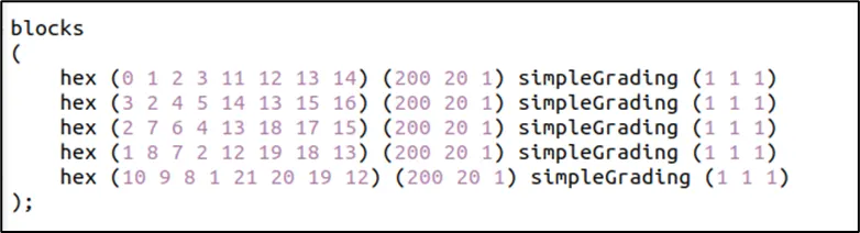
In the above figure hex represents hexahedral mesh and (0 1 2 3 11 12 13 14)represents the faces of block 1 in which(0 1 2 3) is the back face of block 1 and (11 12 13 14) is the front face of block 1.

(200 20 1) represents the number of cells in x,y and z direction respectively.

Afterwards in codes we provide x,y and z coordinates location starting from the vertex (0 0 0),in order to create the geometry let us consider creating the geopmetry using 5 blocks as shown

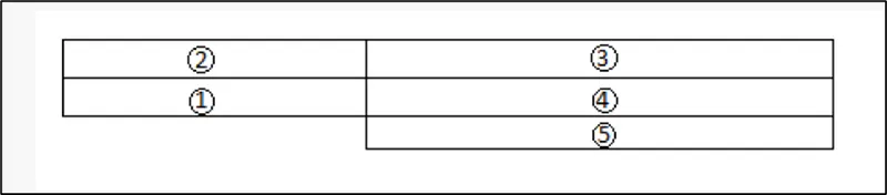
Now,we are going to provide the vertices for each block by refering to the sketch

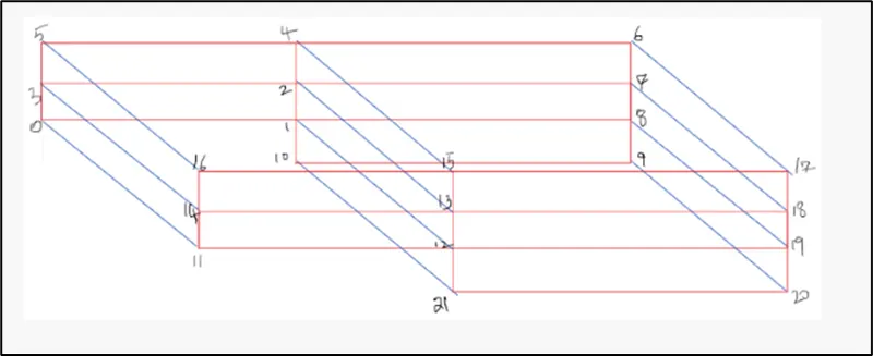
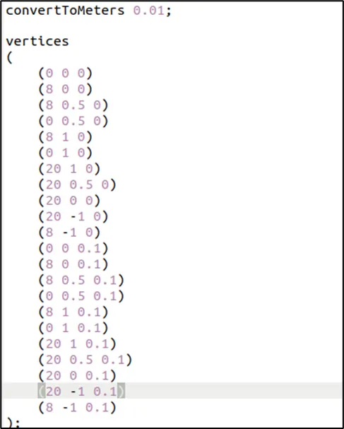
Afterwards we edit the boundary of the geometry by setting the inlet,outlet front and back and fixed walls for the geometry

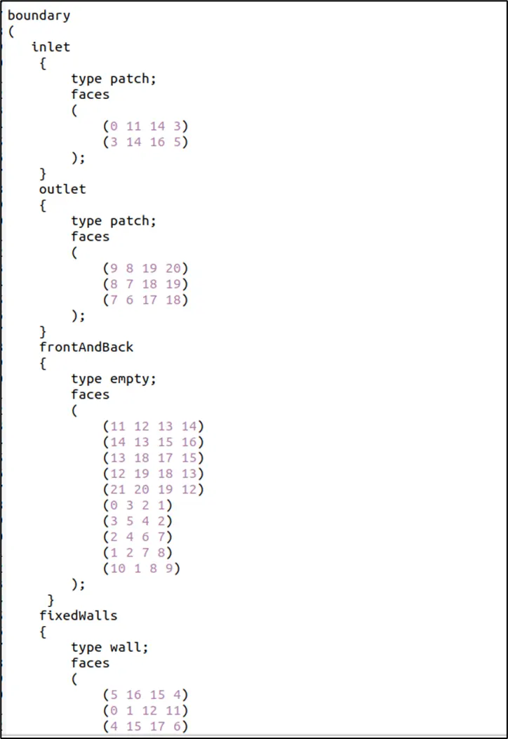
boundary
(
     inlet
     {
       type patch;
       faces
       (
         (0 11 14 3)
         (3 14 16 5)
       );
     }
     outlet
     {
       type patch;
       faces
       (
         (9 8 19 20)
         (8 7 18 19)
         (7 6 17 18)
       );
     }
     fixedWalls
     {
       type wall;
       faces
       (
         (5 16 15 4)
         (0 1 12 11)
         (4 15 17 6)
         (10 9 20 21)
         (10 21 12 1)
       );
     }
      frontAndBack
     {
       type empty
       faces
       (
         (11 12 13 14)
         (14 13 15 16)
         (13 18 17 15)
         (12 19 18 13)
         (21 20 19 12)
         (0 3 2 1)
         (3 5 4 2)
         (2 4 6 7)
         (1 2 7 8)
         (10 1 8 9)

       );
     }

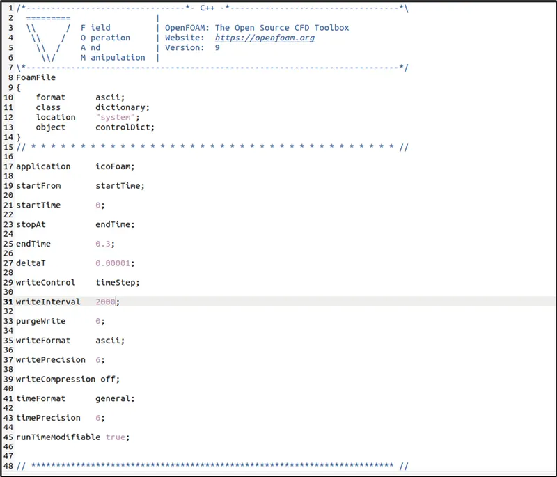
After editing the blockMeshDict file save it and close it,furthermore we are going to edit controlDict file to provide the time limit for the simulation and also choose the value of delta t so that CFL value should be less than 1 for the convergence of the solution.

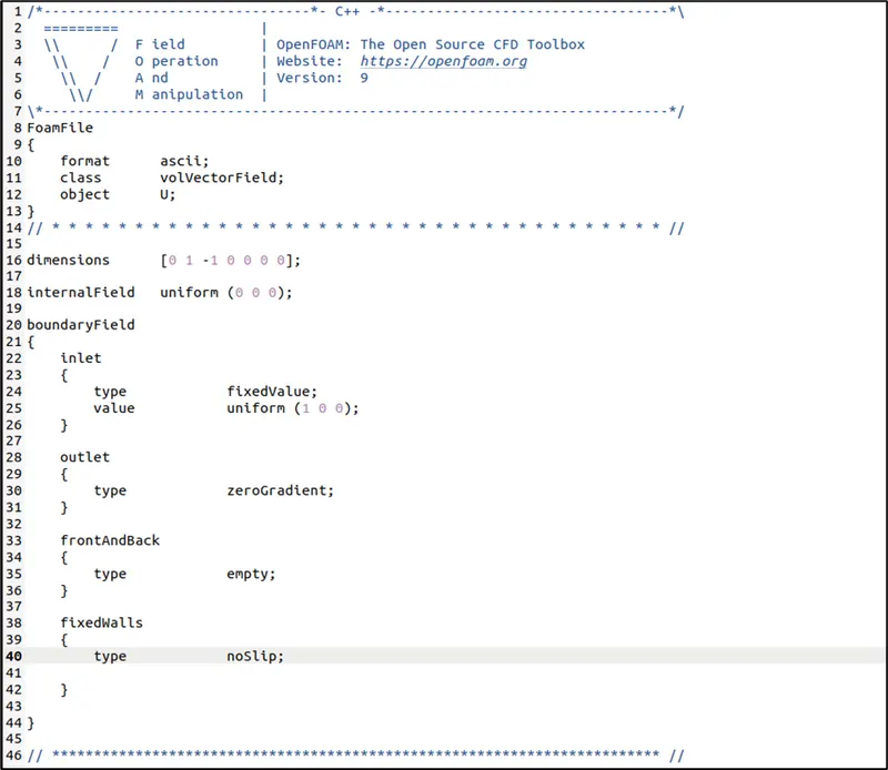
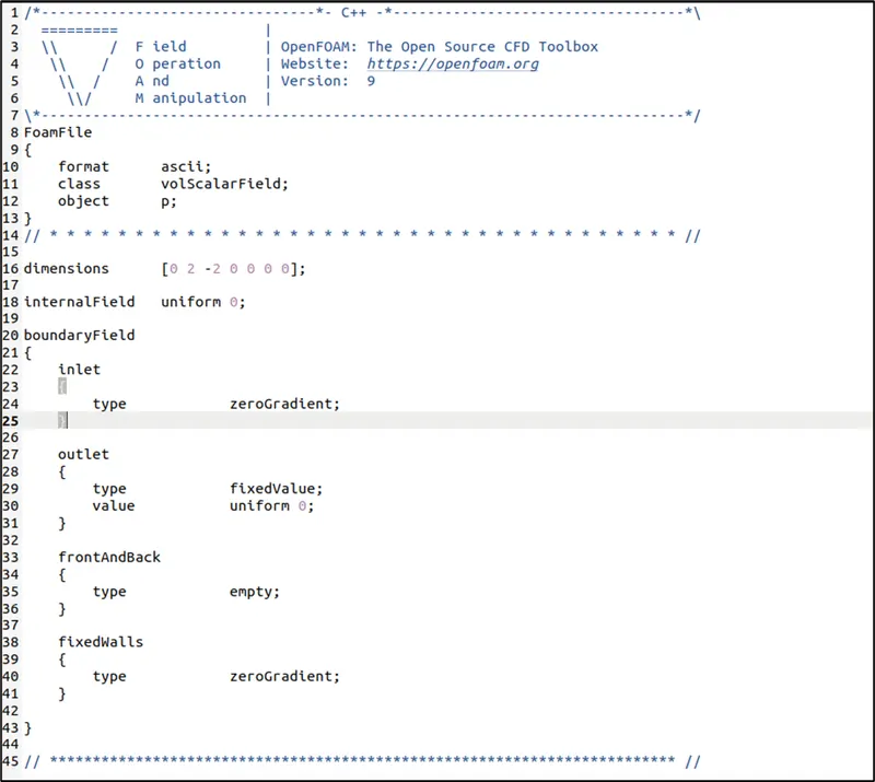
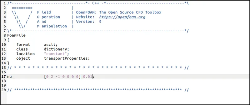
In this case,we have to set initial boundary condition for pressure and velocity at each faces also update the name of boundary same as we changed inlet outlet name in blockMeshDict script file as shown in below code.

INITIAL VELOCITY:

INITIAL PRESSURE:

TRANSPORT PROPERTIES:

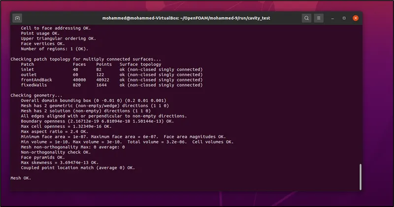
At this point,our problem statement is set,we can now proceed to deploy the mesh using 'blockMesh' command and then 'checkMesh' command to check if there any errors in our mesh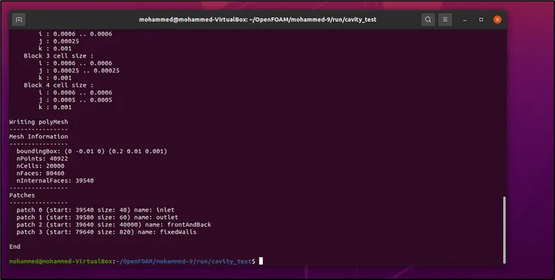

We can now check our mesh by typing paraFoam command

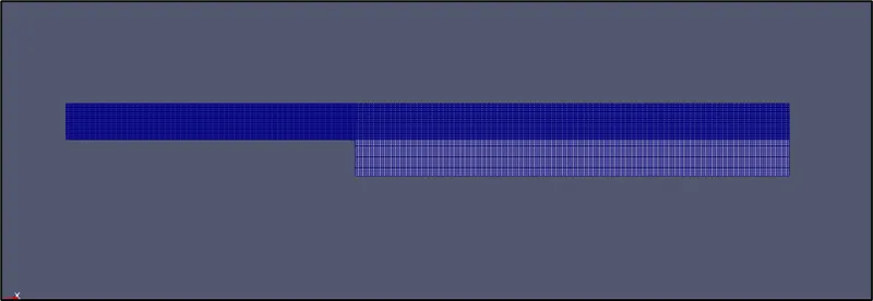
we can improve the mesh flow as it is not uniformly distributed we can make uniform by varying the number of cells in x and y direction in blockMeshdict file

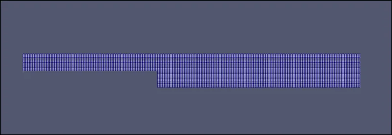
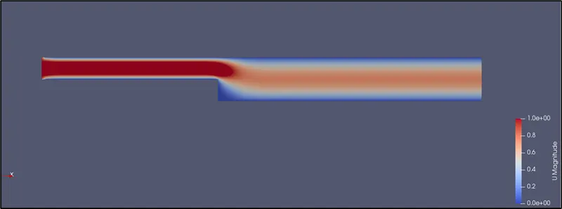
VELOCITY DISTRIBUTION:

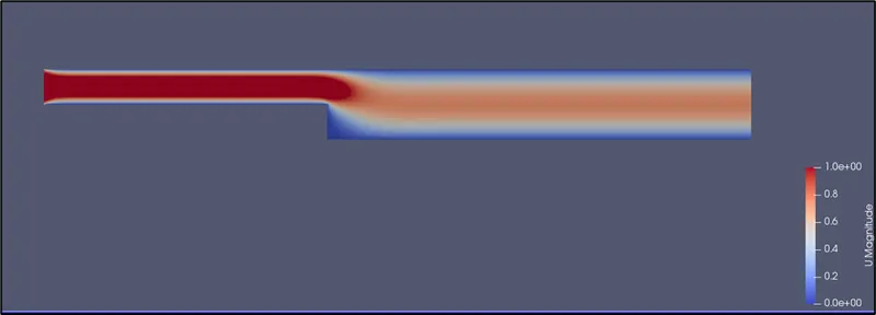
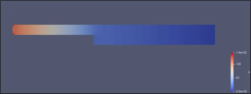
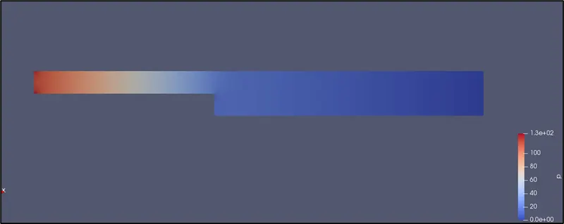
PRESSURE DISTRIBUTION:

VELOCITY PLOT AT 0.085m from the inlet:

CASE 2:

SIMULATION OF BACKWARD FACING STEP WITH GRADING FACTOR OF 0.2:

We can change the grading factor to 0.2 in blockMeshDict file as shown below

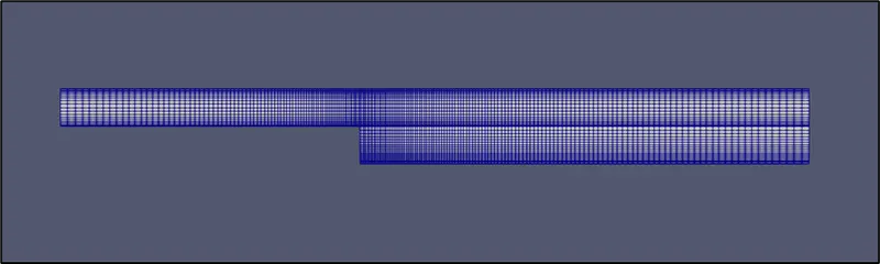
MESH FLOW:

VELOCITY PROFILE:

PRESSURE PROFILE:

VELOCITY PLOT AT 0.085m from the inlet:

• OBSERVATIONS:

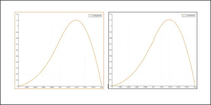
From the above two plots one with orange background is a velocity plot without grading factor and other one us a velocity plot with grading of 0.2,if we take a look at these plots,we can see the plot for velocity without grading factor seems more smooth when compared to other this is because of mesh is fine at step wall along x-axis but very course along y-axis.Therfore we are not getting smooth plot for velocity at 0.085 point at y-axis.To get effective and reliable results,one should know where to use finer grading factor,suppose if we use large number of fine elements,it could use more computational time and also require more computational memory.Therfore use of grading is important,so that we can use fine mesh to capture the flow at boundary wall and obstacles,course mesh at more open areas.