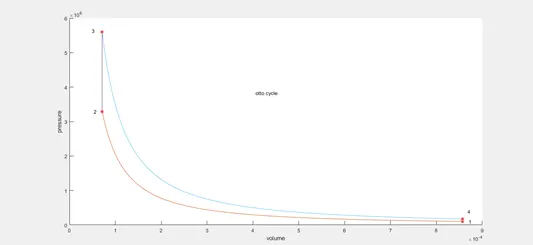
Air Standard Otto Cycle

OTTO CYCLE:

• AIM:

The main aim of this project is to calculate the thermal efficiency of an otto cycle and to plot the p-v diagram using MATLAB programming.

• OBJECTIVE:

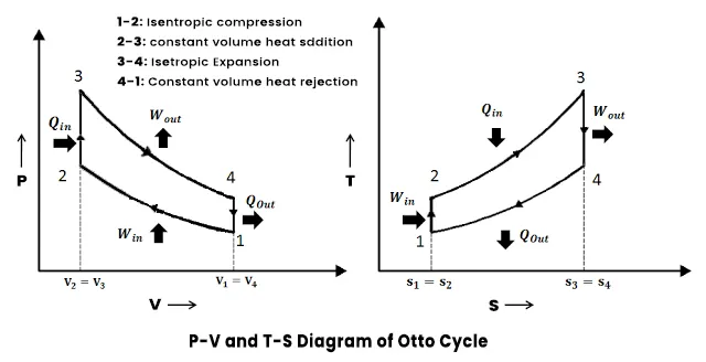
Otto cycle or constant volume cycle,on this cycle petrol engine ,gas and many types of engine work.It is a standard or comparision cycle to the internal combustion engine.The p-v and T-s diagram are shown in the figure.

• THERMAL EFFICIENCY OF OTTO CYCLE:

Let us consider 1kg of air(working substance)

Heat supplied at constant volume = c_v*(t3-t2) c_v = specific heat at constant volume in j/kg-k

Heat rejected at constant pressure = c_v*(t4-t1)

efficiency = workdone/heat supplied

= 1-(t4-t1)/(t3-t2) ............................. (1)

compression ratio c_r = v1/v2

from 1 - 2

As it is isentropic compression p1*v1^gamma = p2*v2^gamma gamma = c_p/c_v

t2/t1 = (v1/v2)^(gamma-1) ........................(2)

from 3-4

As it is isentropic expansion p3*v3^gamma = p4*v4^gamma

t3/t4 = (v4/v3)^(gamma-1)........................(3)

substitute the equation (2) and (3) in equation (1)

EFFICIENCY = 1-1/(C_R)^(GAMMA-1)

This expression is known as air standard or thermal efficiency of an otto cycle.

• EXPLANTION:

1. Bring all the engine geometric parameter values like bore ,stroke,connecting rod ,compression ratio. By which we can able to trace the swept volume and clearence volume.
2. Input the state variable value which is known and calculate the rest by thermodynamic relations.
3. plot the state variables value in P-V diagram.
4. To trace the volume change in isentropic compression (1-2) we have to call a function V_compression = engine_kinematics(bore,stroke,con_rod,c_r,start_crank,end_crank) and then we can get the volume trace during compression in p-v diagram.
5. plot the p-v diagram by plot command and input the state variables and indicate the position by gtext command .

volume trace is calculated by the equation

v/v_c = 1 +1/2*(c_r-1)*(R+1-COS(θ">θθ)-(R^2-sin^2(theta)^1/2)

clear all
close all
clc

%geometric dimensition

bore=0.1;
stroke=0.1;
con_rod=0.15;
c_r=12;

v_s = (pi/4)*bore^2*stroke;
v_c = v_s/(c_r-1);

%state variables 1
gamma = 1.4;
t3 = 2300

p1=101325;
v1= v_s+v_c;
t1 = 500;

constant_c = p1*v1^gamma;
V_compression = engine_kinematics(bore,stroke,con_rod,c_r,180,0)
P_compression = constant_c./V_compression.^gamma

%state variables 2

v2 = v_c;
p2 = p1*c_r^gamma;
t2 = p2*v2*t1/(p1*v1);

%state variables 3 

v3 = v2;
p3 = t3*p2/t2;

constant_c = p3*v3^gamma;
V_expansion = engine_kinematics(bore,stroke,con_rod,c_r,0,180)
P_expansion = constant_c./V_expansion.^gamma

%state variables 4 
v4 = v1;
p4 = p3*(v3/v4)^gamma;
%thermal efficiency

efficiency = 1-(1/(c_r)^(gamma-1))

%plotting

figure(1)
hold on


plot(v1,p1,'*','color','r')
plot(V_compression,P_compression)
gtext('1')

plot(v2,p2,'*','color','r')
plot([v2 v3],[p2 p3])
gtext('2')

plot(v3,p3,'*','color','r')
plot(V_expansion,P_expansion)
gtext('3')

plot(v4,p4,'*','color','r')
plot([v4 v1],[p4 p1])
gtext('4')

gtext('otto cycle')
xlabel('volume')
ylabel('pressure')

The following function code has been called in the above MATLAB programm

function [V] = engine_kinematics(bore,stroke,con_rod,c_r,start_crank,end_crank)
clear all
close all
clc

%inputs

a = stroke/2;
R = con_rod/a
theta = linspace(start_crank,end_crank,180)
v_s = (pi/4)*bore^2*stroke
v_c = v_s/(c_r-1)

%volume trace

term1 = 0.5*(c_r-1);
term2 = R+1-cosd(theta);
term3 = (R^2-sind(theta).^2).^0.5;

V = (1+term1*(term2-term3))*v_c

end

• CONCLUSION:

1. Thermal efficiency of an otto cycle is 62.99% is obtained and p v diagram is plotted.